
Directional Wavelet Transform
2D Continuous Wavelet Transform
All geometric operations in \(2D\) space can be seen as a combination of three operations.
- 1. Translation: Translation in \(2D\) corresponds to translation in \(1D\) space. A translation of vector \(\bar{b}\) is represented as \(\bar{x}-\bar{b}\). \(\forall \bar{x}, \bar{b} \in R^{2}\)
- 2. Dilation : Dilation by a scalar \(a\) is given by \(a\bar{x}\).
- 3. Rotation : Rotation by \(\theta\) which is given by \(r_{\theta}(\bar{x})\) where \(r_{\theta}\) is the usual rotation matrix given by
Let \(s(\bar{x})\) be a \(2D\) signal then the three operations on this signal are given by
\[ s_{\bar{b},\theta,a}(\bar{x})=\frac{1}{a} s(\frac{r_{-\theta}(\bar{x}-\bar{b})}{a}) \]where \(\forall \bar{x}, \bar{b} \in R^{2}, \forall \theta \in [0,2\pi], \forall a \gt 0 \)
If the signal \(s\) is rotation invariant then such a signal is given by
\[ s_{\bar{b},a}(\bar{x})=\frac{1}{a} s(\frac{\bar{x}-\bar{b}}{a}) \]which is \(2D\) equivalent of a \(1D\) translated and dilated signal.
Definition: A \(2D\) continuous wavelet transform of a \(2D\) signal with respect to a \(2D\) wavelet \(\psi_{\bar{b},\theta,a}\) is given by the inner product
\[ S_{\bar{b},\theta,a}= <\psi_{\bar{b},\theta,a}, s> \] \[ S_{\bar{b},\theta,a}=\int_{R^{2}} s(\bar{x}) \psi_{\bar{b},\theta,a}^{*} d^{2}\bar{x} \] \[ S_{\bar{b},\theta,a}=\frac{1}{a}\int_{R^{2}} s(\bar{x}) \psi^{*}(\frac{r_{-\theta}(\bar{x}-\bar{b})}{a}) d^{2}\bar{x} \]The Fourier Transform is given by
\[ \widehat{S}_{\bar{b},\theta,a}=a \int_{R^{2}} e^{i \bar{b} \bar{\omega}} \widehat{s}(\bar{\omega}) \widehat{\psi}^{*}(a r_{-\theta}(\bar{\omega})) d^{2}\bar{\omega} \]\(2D\) CWT Visualization
\(2D\) CWT consists of four variables - two spatial variables represented by \(\bar{b}\), scale parameter \(a\) and rotation parameter \(\theta\). Given that four dimensional visualization is really difficult, the solution is to eliminate one or more variables and then plotting \(S_{\bar{b},\theta,a}\), the \(2D\) wavelet transform.
- 1. Position Representation : The scale and rotation parameter are fixed and CWT is plotted as a function of \(2D\) space.
- 2. Scale-Angle Representation : The position parameters are fixed while we vary scale and angles to plot CWT. Using Polar Co-ordinates : Instead of two-dimensional space parameter \(\bar{b}\) we can use polar representation \((|\bar{b}|,\alpha)\) where \(|\bar{b}|=\sqrt{b_{x}^{2}+b_{y}^{2}}\) known as range and \(\alpha= \arctan{b_{y}/b_{x}}\) which is also known as perception angle. We can use these four parameters to come up other sets of visualizations, namely
- 3. Perception Angle-Scale Representation : We fix range and rotation angle while using perception angle and scale.
- 4. Range-Rotation Angle Representation: Range and Rotation angles are used while fixing scale and perception angle.
- 5. Scale-Range Representation: Scale and Range are used while fixing both angles.
- 6. Angle-Angle Representation: Angles are used while fixing range and scale.
Wavelet Discretization
The issue with \(2D\) continuous transform is same as in the \(1D\) case. It contains a lot of redundant information and a comprehensive continuous transform will be impossibly computationally intensive. We deal with it the same way by discretizing this transform. We choose a grid \(\delta\) to discretize as following
- 1. Discretized Scale Parameter is given as \[ a_{j}=a_{0} \lambda ^{-j} \] where \(\lambda \gt 1\). If we choose dyadic scales then \(\lambda = 2\).
- 2. Discretized Rotation Parameter is uniformly discretized over the entire rotation space \([0,2 \pi) \) as following \[ \theta_{l}=\frac{2l \pi}{L} \] where \(l=[0,1,..., L-1]\) ,\(\forall L \in N\),\(\forall l \in Z\)
- 3. Translation Parameters are discretized using scale and rotation parameters. \[ \bar{b}_{jlm_{x}m_{y}}=a_{0} \lambda ^{-j} r_{\theta_{l}}(m_{x}\beta_{x},m_{y}\beta_{y}) \] \[ \bar{b}_{m}=\bar{b}_{jlm_{x}m_{y}} \]
Wavelet Transform is discretized as following by putting \(a_{0}=1\) and using discretized \(\bar{b}_{m}\)
\[ S_{\bar{b}_{m},\theta_{l},\lambda^{-j}}=\lambda^{j}\int_{R^{2}} s(\bar{x}) \psi^{*}(\lambda^{j}r_{-\theta_{l}}(\bar{x}-\bar{b}_{m})) d^{2}\bar{x} \]The Fourier Transform is similarly given by
\[ \widehat{S}_{\bar{b}_{m},\theta_{l},\lambda^{-j}}=\lambda^{-j} \int_{R^{2}} e^{i \bar{b_{m}} \bar{\omega}} \widehat{s}(\bar{\omega}) \widehat{\psi}^{*}(\lambda^{-j} r_{-\theta_{l}}(\bar{\omega})) d^{2}\bar{\omega} \]Isotropic vs Anisotropic Wavelets
Isotropic Wavelets are rotation invariant wavelets whereas Anisotropic wavelets are directional wavelets. One example of wavelet family that can be used to generate isotropic and anisotropic wavelets is \(2D\) Mexican Hat Wavelet.Anisotropic wavelets can be obtained by stretching isotropic wavelets in a desired direction. This is accomplished by using Anisotropy matrix \(A\)
\[ X_{a}=A X_{iso} \]where \(A= diag[\epsilon^{-\frac{1}{2}},1]\) is a \(2X2\) matrix for \( \epsilon \geq 1\)
Mexican Hat Wavelets are Laplacian of Gaussian functions which are given by
\[ \psi_{m}(x,y)=[2-(x^{2}+y^{2}/\epsilon)]e^{(-\frac{(x^{2}+y^{2}/\epsilon)}{2})} \]\(\epsilon=1\) gives Isotropic wavelet which is plotted in figure below.
\[ \psi_{miso}(x,y)=[2-(x^{2}+y^{2})]e^{(-\frac{(x^{2}+y^{2})}{2})} \]Anisotropic (Rotation Variant) Wavelet is given by using the formula introduced above.
\[ \psi_{\bar{b},\theta,a}(\bar{x})=\frac{1}{a} \psi(\frac{r_{-\theta}(\bar{x}-\bar{b})}{a}) \]Different values of \(\theta\) and scaling parameters \(a\) generate different Mexican hat wavelets. For this example, we use values of \(a=0.8\), \(\theta=3 \pi/4\) and \(\epsilon=5\). It should be noted,however, that these ``stretched'' wavelets only have limited directional selectivity.
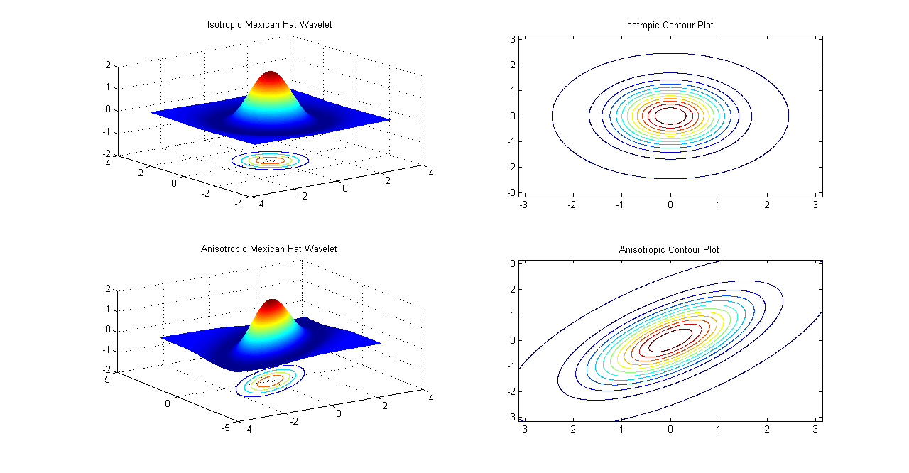
Isotropic and Anisotropic Mexican Hat Wavelets
Directional Wavelet Examples
A wavelet is said to be directional wavelet if its fourier transform is directionally contained in a convex cone in frequency space \(\omega\) with apex at the origin. Thus, anisotropic Mexican Hat wavelet even with its directional selectivity is not a Directional wavelet as it is centered around the origin.
\(2D\) Morlet Wavelet is given by
\[ \psi_{M}(x)=e^{i \bar{k}_{0} \bar{x}} e^{-\frac{1}{2} |A \bar{x} |^{2}}-e^{-\frac{1}{2} |A^{-1} \bar{k}_{0} |^{2}}e^{-\frac{1}{2} |A \bar{x} |^{2}} \]where \(A= diag[\epsilon^{-\frac{1}{2}},1]\) is a \(2X2\) matrix for \( \epsilon \geq 1\) and \(\bar{k}_{0}\) is a \(n-\) dimensional vector corresponding to \(n-\) dimensional \(\bar{x}\) vector. Morlet wavelet is complex and assuming we take values of \(\epsilon = 3\) and \(\bar{k}_{0}= (0,6)\), real and imaginary parts of Morlet can be plotted as shown below.
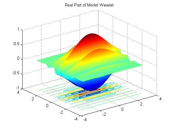
Real part of Morlet Wavelet
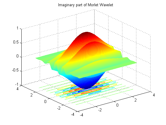
Imaginary Part of Morlet Wavelet
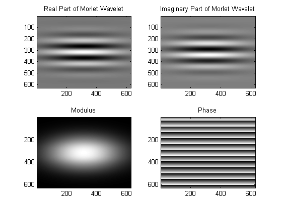
\(2D\) plots of real and imaginary parts along with phase and modulus are also shown. Color white corresponds to highest amplitudes while black corresponds to lowest amplitudes. Phase plot is the most interesting one as it is a collection of straight lines whose intensity varies linearly and periodically in perpendicular direction( to \(\bar{k}_{0}\) ).
Morlet Wavelet Directional properties
In spatial frequency domain, the fourier transform \(\widehat{\psi}_{M}(\omega)\) is centered at \(\bar{k}_{0}\) instead of origin and its directionality depends on anisotropic matrix ,specifically on value of \(\epsilon\). The Fourier Transform is elongated in \(\omega_{y}\) direction in this case. The shape of cone depends on \(\epsilon\) value as greater anisotropy corresponds to narrower cone.
\[ \widehat{\psi}_{M}(\omega)=\sqrt{\epsilon}( e^{-\frac{1}{2} |A^{-1} (\bar{\omega}-\bar{k}_{0} |^{2}}-e^{-\frac{1}{2} |A^{-1} \bar{k}_{0} |^{2}}e^{-\frac{1}{2} |A^{-1} \bar{\omega} |^{2}}) \]The second term is usually small for large values of \(\bar{k}_{0}\) and is therefore ignored.
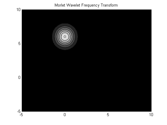
Morlet Wavelet Frequency Transform
Directionality and Separable Filter Banks
Standard \(2D\) DWT has limited directionality as it resolves directions in only three directions- horizontal, vertical and diagonal. \(2D\) Filter Bank Implementation of \(2D\) DWT is shown below

2D Discrete Wavelet Transform
The directional decomposition of Lena image using this filter bank is three-directional with large coefficients in spatial band pass frequency domain aligned in vertical, horizontal and diagonal directions.
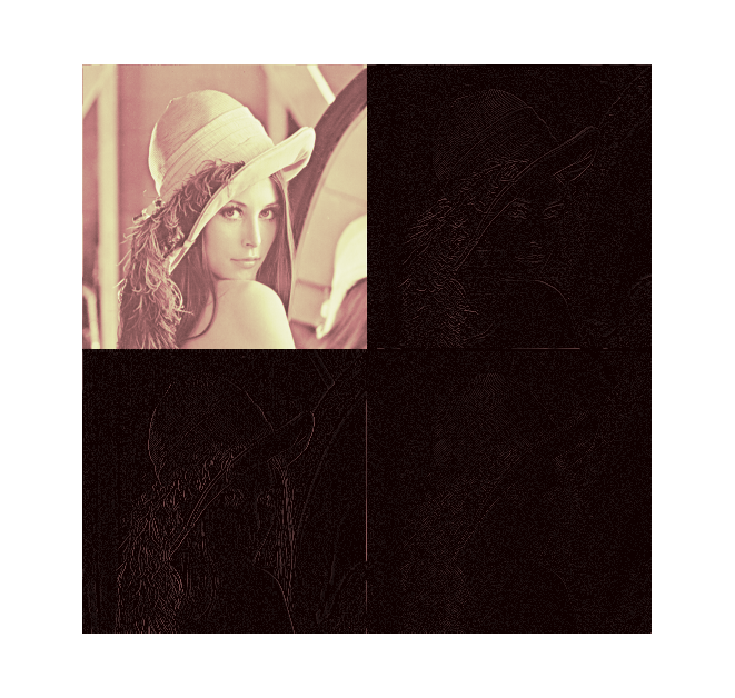
1-Level DWT Decomposition of Lena Image
Standard \(2D\) DWT is isotropic as filtering and sampling operations are performed identically in both horizontal and vertical directions. As we know, there are three wavelets corresponding to three bandpass frequency domains - the low-high band, high-low band and high-high band and as can be seen they have limited directional properties.However, low complexity and ease of implementation means that isotropic separable filter banks are used extensively in practice. The three wavelets corresponding to Haar filters are plotted below.
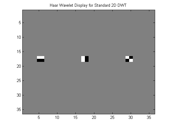
Three Haar Wavelets for 1-level 2D DWT
Anisotropic DWT using Separable Filter Banks
In certain \(2D\) applications it is desirable to detect edges and contours that are aligned at various angles. Standard DWT gives sub-optimal performance in these type of cases.One straightforward and slightly better method is to use anisotropic DWTs that are constructed by using unequal filtering and sampling operations in horizontal and vertical directions. As mentioned this is not an optimal approach but may result in better performance in certain cases. One such example is anisotropic filtering is shown below.
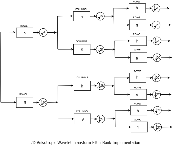
2D Anisotropic Discrete Wavelet Transform Example
It uses three-levels of filtering and subsampling operations at the analysis and synthesis( not shown) side which means higher complexity than the standard case which uses two levels of operations. In this particular case, horizontal filtering and subsampling is followed by vertical filtering(and subsampling) and the third level consists of horizontal filtering(and downsampling) so for every stage of DWT operations, a \(2D\) signal is divided into \(8\) subimages- one low pass subimage and \(7\) band pass subimages. This can be seen for ``Lena'' Image.
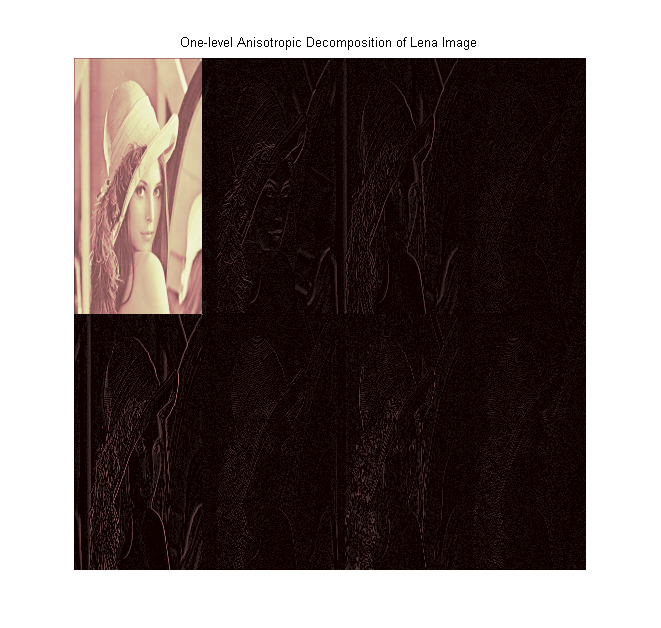
1-Stage Anisotropic DWT Decomposition of Lena Image
As can be seen the \(7\) bandpass images accentuate different directional elements of the image. This directionality property of this particular Anisotropic DWT can be further studied by plotting wavelets associated with each of the seven bandpass subimages for one stage of DWT decomposition. As in the standard DWT case, these seven wavelets are plotted corresponding to Haar wavelet filters.
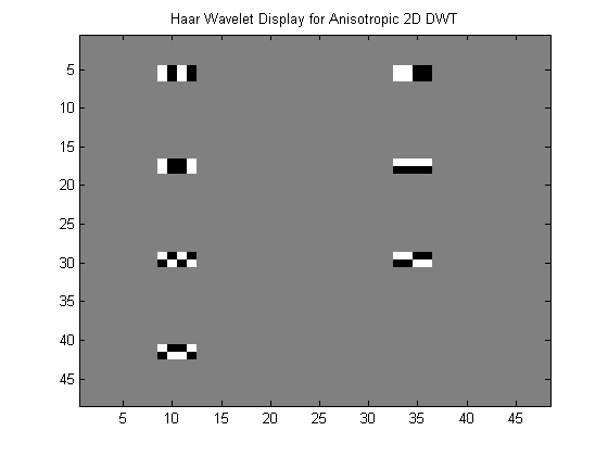
Seven Haar Wavelets for 1-Stage 2D Anisotropic DWT
As can be seen from the wavelet plots , while the directional properties are better in this case, such a configuration will still struggle to isolate edges and contours arbitrary aligned in the \(2D\) space.