Wavelets and Image Compression
Image Approximation
The ideas for one dimensional signal approximation using fewer coefficients were developed previously. These ideas can be extended to \(2D\) signals, ie. images. It was also shown that Nonlinear Approximation results in better performance than linear approximation.Recall that Nonlinear approximation consists of selecting \(M\) largest coefficients instead of the first \(M\) coefficients as in Linear case. Nonlinear approximation performance for wavelets is significantly better than in the linear case as quite a few large coefficients exist at every scale of signal decomposition. In the images case, we'll stick with nonlinear approximation owing to its superior performance.
Approximation Example: Lena Image Approximation using \(1/50\) coefficients
As an example of approximation , consider the Lena image approximation using Fourier Transform and Wavelet Transform. Algorithms are same as in the \(1D\) case.

Original 512X512 Lena Image
In Fourier case, we take the fourier transform of the image and retain only the largest one out of fifty coefficients while setting the rest equal to zero and then we reconstruct the image using only largest \(2\%\) coefficients . The reconstructed image is shown below.

Lena Image Fourier Approximation using only largest 2% coefficients
Next we repeat the same approximation process with Wavelet Method. We take \(J=4\) stage Discrete Wavelet Transform (derived from Db2 wavelets) of the Lena image, choose the largest \(\frac{1}{50}\) coefficients while setting the rest equal to zero. Then the Inverse Discrete Wavelet Transform is taken using these new coefficients. The resulting Image is shown below and is seen to be superior reconstruction compared to the Fourier case.

Lena Image Wavelet Approximation using only largest 2% coefficients
Information Theory Background
Let us assume that system source is a discrete and finite consisting of N symbols and is given by \(S\) also known as alphabet.
\[ S=[s_{0},s_{1},....,s_{N-1}] \]Let \(X=[x_{0},x_{1},....,x_{i},....\) be a collection of output sequence where each output \(x_{i}\) is taken from the set \(S\). The probability that this system outputs the \(kth\)symbol \(s_{k}\) is given by \(p_{k}\) where
\[ \sum_{k=0}^{N-1} p_{k}=1 \]as there are only \(N\) symbols.
Self-Information: We define information content \(I_{k}\) of each symbol based on its probability of being the output. It is given by
\[ I_{k}=-\log_{2}(p_{k}) \]and is measured in bits. If \(p_{k}=1\) or the symbol occurs every time then the information content of such a certain event is zero. On the other hand if the event is impossible \(p_{k}=0\) then the information content of such an event is \(\infty\). More realistically, the likelier an event , less information is needed to define the event. On the other hand, unlikley events carry more information.
Source Entropy: is defined as expected value of self-information.
\[ H(S)=E\{I_{k}\}=-\sum_{k=0}^{N-1} p_{k}\log_{2}(p_{k}) \]\(H(S)\) is measured in bits per symbol and is maximal for flat probability distribution, ie., if each symbol is equally probable \(\frac{1}{N}\) then \(H(S)=\log_{2}(N)\). Smaller source entropy can be obtained if probability distribution isn't flat.
Average Bit rate \(R_{x}\): Let \(l_{k}\) be the length of the code associated with \(kth\) symbol with output probability \(p_{k}\) then the Average Bit Rate \(R_{x}\) is given by
\[ R_{x}= \sum_{k=0}^{N-1} p_{k}l_{k} \]The objective of good coding is to minimize the average bit rate for a given information source.Also, \(H(S)\) sets the lower bound on average bit rate so \(R_{x}\) for a particular coding scheme can be measured against source entropy.
Prefix Code: One important condition for any good code is that no codeword can be a prefix of another codeword. As an example consider a code with following codewords
\[ c_{1}=1 , c_{2}=11 , c_{3}=10 , c_{4}=101 \]Consider a sequence \(1011\). It can be written as both \(c_{4}c_{1}\) and \(c_{3}c_{2}\) which will not work at the decoder stage. The solution is to generate codes using prefix binary tree.Each node of the tree has only one input branch and no more than two output branches with left branch labeled as \(0\) branch and right branch as \(1\). The binary tree ends in \(K\) leaves each corresponding to a unique codeword. In this case, length \(l_{k}\) of each codeword is given by the number of branches from the node to the \(kth\) leaf.
Huffman Coding
Premise of Huffman coding is that more probable a symbol, the shorter its length should be. If \(P(s_{i}) \lt P(s_{j})\) then \( l_{j} \ge l_{i}\). Huffman Codes are constructed in \(4\) steps as following.
- 1. Arrange symbol probabilities in decreasing order. \( p_{0} \ge p_{1} \ge .... \ge p_{N-1} \). The symbols \(s_{k}\) form the \(kth\) leaf nodes in binary tree \(T\).
- 2. Combine the two nodes with lowest probability to form a new ``parent'' node. The new node will have the probability. \[ p_{12}=p_{1}+p_{2} \] where \(p_{1}\) and \(p_{2}\) are the probabilities of the two ``children'' nodes while \(p_{12}\) is the probability of the new ``parent'' node.We assign \(0\) value to the branch connecting parent node to child node with probability \(p_{1}\) and \(1\) value to the branch connecting parent node to child node with probability \(p_{2}\).
- 3. Update binary tree \(T\) by replacing the two children nodes with the parent node. If the tree has more than one node after updating repeat step \(2\). If there is only one node left, it is the root node.
- 4. Codeword of each \(s_{k}\) can be obtained by traversing from root node to the \(kth\) leaf node.
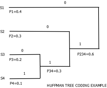
Huffman Coding Example

Huffman Coding Example
The codeword can be obtained as in \(4\). We get
\[ s_{1}=0 , s_{2}=10 , s_{3}=110 , s_{4}=111 \]The average bit rate is found by using
\[ R_{x}= \sum_{k=0}^{N-1} p_{k}l_{k} = 0.4 * 1 + 0.3 * 2 + 0.2 * 3 + 0.1 * 3 = 1.9 \]The source entropy is calculated using
\[ H(S)=E\{I_{k}\}=-\sum_{k=0}^{N-1} p_{k}\log_{2}(p_{k}) \] \[ H(S)=-[0.4*log_{2}(0.4)+0.3*log_{2}(0.3)+0.2*log_{2}(0.2)+0.1*log_{2}(0.1)] = 1.846 \]The average bit rate is a bit higher than source entropy but still gives better results than usual bit coding which corresponds to \(2\) bits per symbol for this example.
Arithmetic Coding
Drawbacks of Huffman Coding
- 1. It assigns integer length to each symbol.
- 2. It depends on the source probabilities. If the system is adaptive with probabilities that change, the code has to be reset each time.
Basis of Arithmetic Coding:Consider a binary sequence \(B = 100111011\). We can convert it into a decimal number \( 0 \leq v \leq 1\) by expressing it as \( 0.100111011_{2} \), which is equal to \( v = 0.615234375_{10} \). In other words, regardless of how large a number is, it can be mapped to \( [0,1)\). In arithmetic coding, we create a sequence of nested intervals
\[ \phi_{k}(S)= [a_{k},b_{k}) \]where \(a_{k}\) and \(b_{k}\) are real numbers and
\[ 0 \leq a_{k} \leq a_{k+1} , b_{k+1} \leq b_{k} \leq 1 \]Alternatively, we can represent each interval in form of base (lowest value \(b\)) and the length of the interval \(l\).
\[ |b,l \gt \]Arithmetic coding Algorithm
- 1. Find probability distribution and cumulative distribution of the source inputs.
- 2. Find \( |b_{0},l_{0} \gt \) which is the initial value. Typically, initial values correspond to \( |0,1 \gt \) or the entire length of the probability distribution.
- 3. Corresponding to the first input value, find \( |b_{1},l_{1} \gt \). These two values are calculated as follows
\[
|b_{k},l_{k}\gt = |b_{k-1}+c(s_{k})l_{k-1}, p(s_{k}) l_{k-1} \gt
\]
where the \(kth\) input corresponds to one value in the set of source symbol and \(p(s_{k})\) and \(c(s_{k})\) are respectively the probability and cumulative density functions associated with the source symbol.
- 4. Corresponding to every new input value we update the base sequence and its length by using \(3\).
- 5. Once the last input value, say \(nth\) value is read, we have a sequence \( |b_{n},l_{n} \gt\). This interval is used to encode a binary number choosing a value that corresponds to shortest binary code. This value is the arithmetic encoded value.
Example: Let us consider a source consisting of four symbols with probability and cumulative distribution given as
\[ p=[0.2 , 0.5 , 0.2 , 0.1] \] \[ c=[0 , 0.2 , 0.7 , 0.9 , 1] \]Let us consider an input sequence \(S= [ 2 , 1] \). Corresponding to first value \(2\), we have \(p(s_{1}) = 0.2 \) and \(c(s_{1}) = 0.7 \). Calculating
\[ |b_{1},l_{1}\gt =|b_{0}+c((s_{1})l_{0},p(s_{1}l_{0}\gt = |0.7,0.2 \gt \]Corresponding to second value \(1\), we have \(p(s_{2}) = 0.5 \) and \(c(s_{2}) = 0.2 \). Calculating
\[ |b_{2},l_{2} \gt =|b_{1}+c((s_{2})l_{1},p(s_{2}l_{1}\gt = |0.74,0.10 \gt \]If we are transmitting only two values, this encoding gives us a choice to generate shortest binary number in the range \( 0.74-0.75\). Minimum number of bits needed for encoding purposes are given by
\[ B_{m}= -\log_{2} (l_{n}) \]\(B_{m}\) is rounded up to the nearest integer. This coding is especially effective for a large chain of input values as all inputs are encoded together as a block with trade off being a more complex implementation is needed to generate the codeword.
Decoding
Although some overhead is needed, decoding depends solely on binary string \(v\). The decoding is done as follows
- 1. Define \(v_{1}=v\).
- 2. The output value is given as follows: \[ s_{k}^{o}={s:c(s) \leq v_{k} \leq c(s+1)} \] Essentially, we map \(s_{k}^{o}\) on the symbol interval based on value of \(v_{k}\) and \(c(s)\) is the cdf of the symbol value corresponding to \(s\). As is obvious , the decoder needs the probability distributions (pdf and cdf) of the source symbols in order to decode the binary string. This adds to the overhead but it amounts to small value in case of large scale data transmission.
- 3. Update Value of \(v_{k+1}\) as following: \[ v_{k+1}=\frac{v_{k}-c(s_{k})}{p(s_{k})} \]
- 4. One issue with arithmetic coding is that the recursion formula in \(3\) will keep going on regardless of the number of input values so some overhead is needed to tell the decoder where to stop. Typically, overhead can consist of number of input values \(N\) along with the binary string \(v\) and probability distributions. The decoder can then decode for \(N\) output values. If \( k == (N+1)\), the decoder stops else we go back to step \(2\).
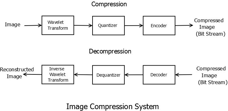
- 1. Wavelet Transform Stage: The advantage of wavelet transform stage can be seen in the image approximation example shown earlier. The image is transformed into a set of coefficients most of which are close to zero and can be eliminated which results in substantial reduction in amount of data that needs to be encoded. Thresholding is done in order to further reduce the number of significant coefficients. Various algorithms will be covered in the next section.
- 2. Quantizer: Quantization step is usually skipped if one is aiming for lossless compression, eg. medical imaging systems, as quantization is non-invertible. In case of lossy compression, quantization is done to reduce precision of the values of wavelet transform coefficients so that fewer bits are needed to code the image. For example if the transform coefficients are 64- bit floating point numbers while a compression of the order of 8 bits per pixel is required then quantization is necessary.
- 3. Encoding: Encoding was covered in previous chapter. Basically, quantized wavelet transform coefficients are coded so that fewest number of bits are required. Huffman coding, arithmetic coding and their variants are usually used in these systems.
- 1. POS : Positive Significant. The absolute value of coefficient is greater than the threshold and coefficient has positive sign.
- 2. NEG : Negative Significant. The absolute value of coefficient is greater than the threshold and coefficient has negative sign.
- 3. ZTR : Zero Tree Root. The coefficient value is \(0\) and so are the values of each of its descendants.
- 4. IZ : Isolated Zero. The coefficient value is \(0\) but the descendant values are not all zero.
- 1a. Set wavelet transform mean to zero by subtracting the mean from each sample value. We should end up with positive and negative values instead of just positive values.
- 1b. Sign bits are assigned based on whether the coefficient is greater than or less than zero. These sign bits are transmitted in addition to bit plane encoded bits.
- 2. Choose Initial threshold \(T_{0}\). It is usually chosen as \[ th=floor(\log_{2}(|y|_{max})) \] \[ T_{0}=2^{th} \] where \((|y|_{max})\) is the largest coefficient value as mentioned earlier.
- 3. Significance Pass: In which we find the significant bits in each iteration. They are POS (P) or NEG (N). Insignificant bits are either ZTR(Z) or IZ(I).
- 4. Refinement Pass: All coefficients are set to zero and then we systematically assign bit values only to significant bits. This is done by comparing the coefficient values of POS (P) and NEG (N) with the threshold. If they are greater than the threshold, the output bit is \(1\) and we subtract the threshold value from the absolute coefficient value and the updated coefficient value is stored in the coefficient map.
- 5. Threshold is updated \(T_{k}=T_{0}2^{-k}\) for \(k=1,...,K\)
- 6. Repeat steps 3-5 until either all \(K\) bit planes are finished or the process is terminated early if less accuracy is needed.
- 1. Biorthogonal \(9/7\) Wavelet Transform: It introduces quantization error as coefficients are non-integer.
- 2. Biorthogonal \(5/3\) Wavelet Transform.
- 1. Color Component Transformation and Tiling : \(RGB\) image is transformed into either \(YC_{B}C_{R}\) or \(YUV\). this transformed image is then divided into blocks(tiles), each of which is processed separately.
- 2. Wavelet Transform:\(N\) level dyadic transform is performed on each tile using either \(9/7\) or \(5/3\) biorthogonal wavelets.
- 3. Scalar Quantization and Partition: Scalar Quantization is used to reduce complexity at the cost of some loss of quality. Packet partitioning is done to transform each quantized subband into a set of non-overlapping rectangles.
- 4. Block Coding: Code blocks are formed using non-overlapping rectangles. Each code block is encoded separately using arithmetic coding of bit planes. Bit plane coding is done in three passes- significance, refinement and clean up. In case of lossless coding, all bit planes need to be coded and transmitted. These bit planes are then encoded using arithmetic coder.
Wavelet Image Compression System

Wavelet Image Compression System
Wavelet Compresser broadly consists of three stages.
Wavelet Transform Stage
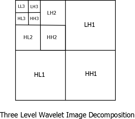
Image Decomposition in terms of two level filtering can be shown as in the next figure. \(LL_{d}\) represents Low-Low pass filtered image at the decomposition level \(d\). \(LH_{d}\), \(HL_{d}\) and \(HH_{d}\) represent Low-High pass filtered image, High-Low Pass filtered image and High-High pass filtered image respectively at decomposition level \(d\). The \(2D\) filter bank is also shown here.

Image Decomposition

2D DWT Filter Bank Implementation
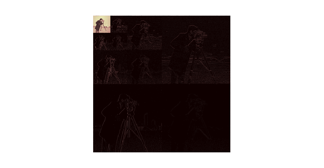
Three level decomposition of an image (cameraman) is given in the figure below.

Image Decomposition
In the figure above, large coefficients are shown by color pink while negligible coefficients are depicted by black and dark shades. The \(LL_{3}\) image is the one containing most significant coefficients while higher frequency image segments have very few large coefficients as most of their coefficients are either zero or nearly zero. Additionally, it can be seen that there is a spatial relationship between coefficients at different decomposition levels.
Zero-Tree Coding
If we look at coefficients in ,say, \(LH_{d}\) subimage and compare them to coefficients in \(LH_{d-1}\), it is seen that there is a spatial relationship across scales. For example, there are a bunch of zero coefficients near the cameraman's shoulder (high coefficient region ) and it is replicated across scales in \(LH\) subimages. Same is true for \(HL_{d}\) and \(HH_{d}\) subimages. This multiscale dependency is the basis of zero-tree coding. For every coefficient at coarse scale there are 4 ``children'' at the next finer scale, ie. one \(HL_{d}\) coefficient is the ``parent'' of four coefficients in \(HL_{d-1}\) and ``grand parent'' of 16 coefficients in \(HL_{d-2}\). The finest scale coefficients don't have any children.
Embedded Zero-Tree Wavelet(EZW) Coding
J.M. Shapiro introduced EZW coding in his 1993 paper. EZW makes use of zero-trees and is a progressive encoding system, ie., as more bits are added the system becomes more accurate.Coding is done in multiple passes. Large coefficients are most important but the way zero-tree deals with smaller coefficients is what makes EZW so effective.
Algorithm
Initial threshold \(T_{0}\) is chosen based on the largest coefficient \(|y|_{max}\)
\[ \frac{|y|_{max}}{2} \lt T_{0} \lt |y|_{max} \]We also define \(T_{k}\) where \(T_{k}=T_{0}2^{-k}\), \(k=0,1,...,K-1\) and is used to update threshold value with every pass.
Let us assume that we are compressing an \(NXN\) image. This image is coded using \(K+1\) binary arrays( bit planes). First bit plane consists of sign bit, the second represents the Most Significant Bit of each coefficient and so on. This process can be terminated at any bit plane \( n \lt K\) but larger the number of bits that are encoded, more accurate the coding is.
Significance Pass: Coefficients are scanned from \(LL_{d}\) down to \(HH_{1}\) in order and it is ascertained whether they are significant or insignificant. An example of a significance pass and labeling can be as following-
We can use \(4\) labels to define coefficients
Refinement Pass : Once we have labeled coefficients, the next pass is used to code the bit values. Each significant bit is compared with updated threshold value \(T_{k}\), ie. , \(T_{1}=T_{0}/2\) and so on in successive passes. If it is greater than \(T_{k}\) then a bit value \(1\) is the output, otherwise \(0\) is the output.
Full Algorithm
JPEG2000 Wavelet Standard
JPEG2000 uses two wavelet transforms. Both are biorthogonal but only one is ``reversible'' as it uses only integer coefficients.
JPEG2000 Coder Basics
For more details on JPEG2000, see the references.
