Discrete Wavelet Transform
Discrete Wavelet Transform was introduced previously with translation and dilation steps being uniformly discretized.
$$\psi_{m,n}(t)=a^{\frac{-m}{2}}\psi(a^{-m}t-n)$$To make computations simpler and to ensure perfect or near-perfect reconstruction, Dyadic Wavelet Transform is utilized. In the dyadic case \(a\) is chosen to be equal to \(2\) which yields the following translation- dilation equation.
$$\psi_{j,n}(x)=2^{\frac{-j}{2}}\psi(2^{-j}x-n)$$,where \(j\) gives the level of scale and n gives the translation where \(j,n\in\)\(Z\). As noted previously, wavelet functions \(\psi(t)\) are bandpass so even with dyadic scaling they cannot cover the entire spectrum so low pass scaling functions \(\phi(t)\) are introduced. Therefore, wavelet coefficients of a function over scales \( j_0 \leq j \leq J \) are then given by
Let there be functions \(\tilde{\phi_{j_0,n}}\) and \(\tilde{\psi_{j,n}}\) such that function \(f(x)\) can be reconstructed from its wavelet coefficients using following equation
The ease with which dyadic Inverse Discrete Wavelet Transform (IDWT) can be constructed makes it ideal for a number of signal processing and image processing applications where reconstruction is absolutely critical(eg., Image compression). More on Inverse DWT using filter banks in next few chapters when this topic will be revisited.
DWT Implementation
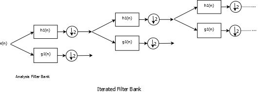
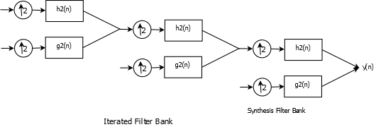
DWT is implemented using decimated filter banks and this implementation is a major reason why DWT has become so popular in DSP and other fields. The concepts behind this implementation will be developed over next few sections but we'll start with the implementation here with results displayed using Matlab.

Filter Bank Implementation of DWT

Filter Bank Implementation of IDWT
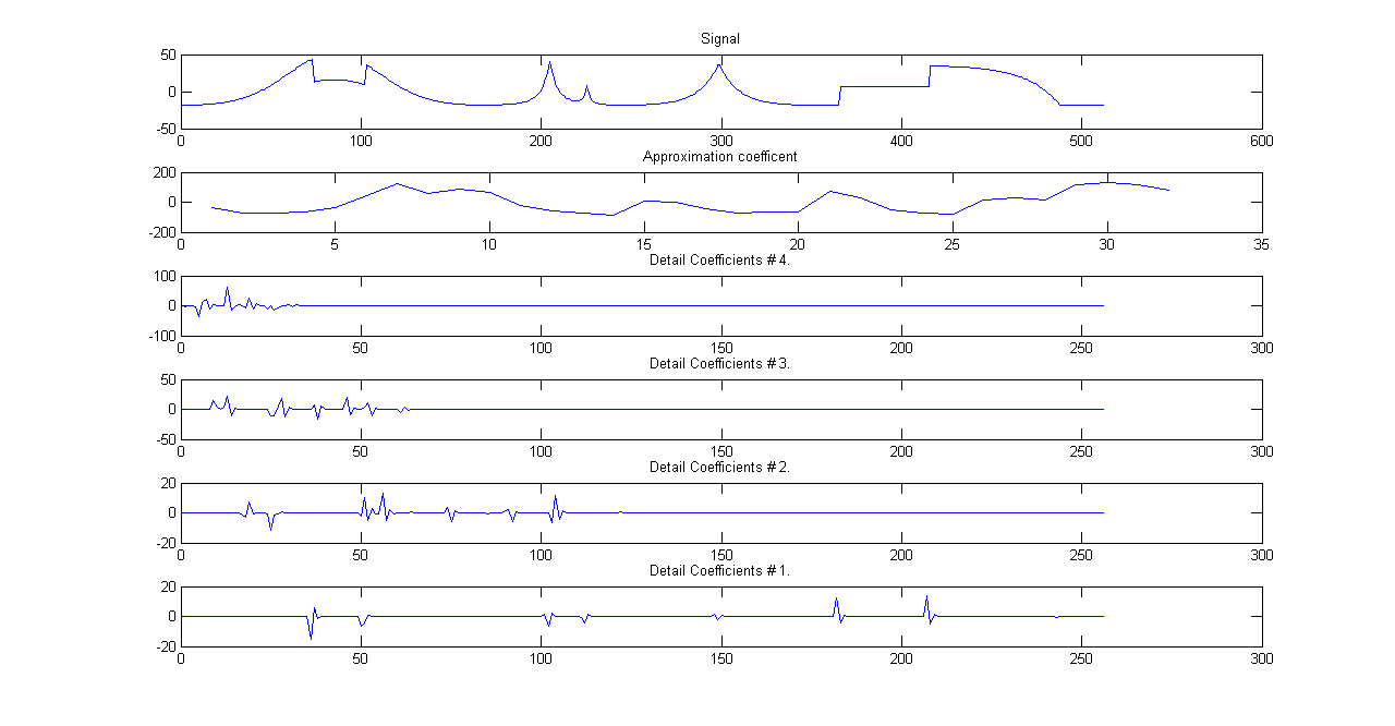
The figures show DWT and Inverse DWT implementations using iterated and decimated filter banks. Consider DWT, at each stage the signal is convolved with low pass and high pass filters and the result is decimated by \(2\). Decimation is necessary in order to keep the system non-redundant as the number of coefficients will, otherwise, double at every stage. The downside is that decimation introduces shift variance.More on this later. For now, we'll pass a signal through the filter bank shown in the first signal and analyze it at every stage. Let us say that the signal is decomposed through \(4\)-levels of the filter banks. At the fourth stage, we have two sets of coefficients- Approximation coefficients corresponding to low pass filter and Detail coefficients corresponding to high pass filtering. Since the low pass approximation coefficients at stages \(1\) through \(3\) are decomposed we'll only consider the detail coefficients at these three stages.At every stage, higher frequency components are peeled off the signal and we are left with a smoother version of the original signal. The analysis is shown in figure.

DWT Analysis of a given signal
