
Steerable Pyramid
Theory of Steerable Filters
Steerable Filters are a class of oriented filters that can be expressed as a linear combination of a set of basis filters. As an example, let us consider isotropic Gaussian filter \(G(x,y)\).
\[ G(x,y)=e^{-(x^{2}+y^{2})} \]First derivative of \(G(x,y)\) is given by \(G_{1}\) and let \(G_{1}^{\theta}\) be the first derivative rotated by an angle \(\theta\) about the origin. In \(x\) direction the angle \(\theta=0^{\circ}\) and in \(y\) direction, \(\theta=90{\circ}\).
\[ G_{1}^{0{\circ}} = \frac{\partial G}{\partial x} \] \[ G_{1}^{0{\circ}}=-2x e^{-(x^{2}+y^{2})} \]and
\[ G_{1}^{90{\circ}} = \frac{\partial G}{\partial y} \] \[ G_{1}^{90{\circ}}=-2y e^{-(x^{2}+y^{2})} \]In \(2D\) space \(G_{1}^{0{\circ}}\) and \(G_{1}^{90{\circ}}\) are seen to span the entire space and are the basis filters. An arbitrarily oriented first derivative filter can be expressed as a linear combination of these two filters.
\[ G_{1}^{\theta{\circ}}=G_{1}^{0{\circ}} cos(\theta) + G_{1}^{90{\circ}} sin(\theta) \]For \(\theta=30{\circ}\), the three filters can be plotted as below
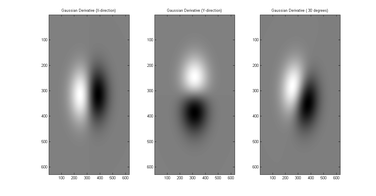
Gaussian First Derivative Filters oriented a) in x-direction b) in y-direction and c) at 30{\circ} about the origin
The first derivative of Gaussian is also an edge detection filter which smooths the \(2D\) signal and then computes the gradient. Having an oriented version of this filter helps in isolating oriented edges and contours. Convolution of an Image \(I\) with an oriented Gaussian first derivative filter \(G_{1}^{\theta{\circ}}\) can be given by
\[ I_{o}^{\theta{\circ}}=G_{1}^{\theta{\circ}}* I \] \[ I_{o}^{\theta{\circ}}=(G_{1}^{0{\circ}}*I) cos(\theta) + (G_{1}^{90{\circ}}*I) sin(\theta) \]or,
\[ I_{o}^{\theta{\circ}}= I_{o}^{0{\circ}} cos(\theta) + I_{o}^{90{\circ}} sin(\theta) \]Convolution of a simple symmetric image with different values of \(\theta\) is shown below.

An Image Convolved with oriented Gaussian first derivative filter
The same plot with an edge detection( gradient computation) point of view is also shown below.
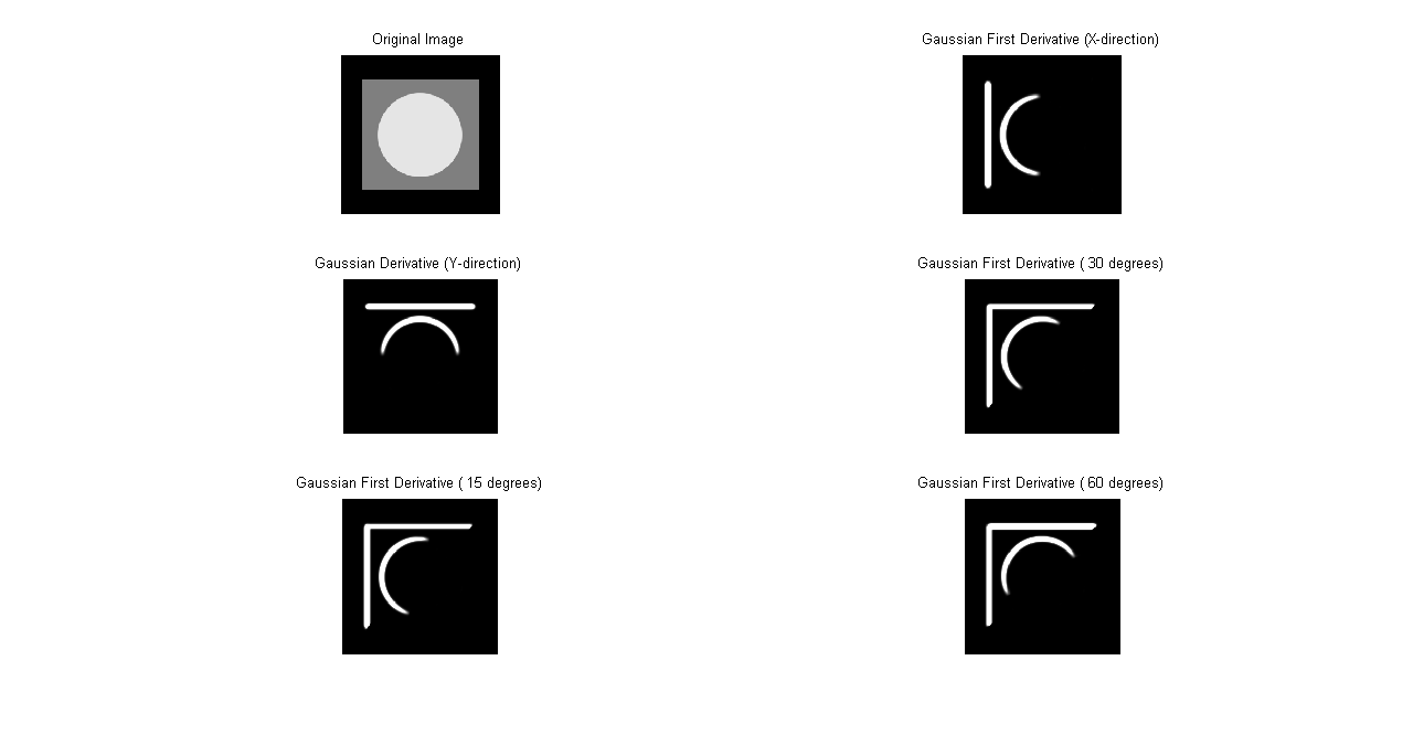
Edge Detection:Image convolved with oriented Gaussian first derivative filters a) original Image, oriented b) in x-direction, c) in y-direction, d) at 30{\circ}, e) 15{\circ}, f) 60{\circ}
Adelson and Freeman Steerability Theorems
Adelson and Freeman proved three theorems in their 1991 paper and these theorems form the basis of Steerable filters and wavelets. A function \(f(x,y)\) steers given the steering condition
\[ f^{\theta}(x,y)= \sum_{j=1}^{M} k_{j}(\theta) f^{\theta_{j}}(x,y) \]where \(f^{\theta_{j}}(x,y)\) are \(M\) basis functions and \(k_{j}(\theta)\) are steer coefficients for a given orientation \(\theta\). \(f(x,y)\) is usually represented in polar coordinates as \(f(r,\phi)\) where \(r=\sqrt{x^{2}+y^{2}}\) and \(\phi=tan^{-1}(y/x)\).
Theorem 1 : Steering condition holds if and only if \(k_{j}(\theta)\) are solutions of following equations
\[ \left(\begin{array}{ccc} 1 \\ e^{i\theta} \\ . \\ . \\ e^{iN \theta} \end{array}\right)=\begin{bmatrix} 1 & 1 & . & 1 \\ e^{i \theta_{1}} & e^{i \theta_{2}} & . & e^{i \theta_{M}} \\ . & . & . & . \\ . & . & . & . \\ e^{iN \theta_{1}} & e^{iN \theta_{2}} & . & e^{iN \theta_{M}} \end{bmatrix} \left(\begin{array}{ccc} k_{1}(\theta) \\ k_{2}(\theta) \\ . \\ . \\ k_{M}(\theta) \end{array}\right) \]The polar coordinate representation of steerable function can be expanded as
\[ f(r,\phi)=\sum_{n=-N}^{N} a_{n}(r) e^{in \phi} \]Theorem 2 : Let \(T\) be the number of positive or negative frequencies for which \(a_{n}(r) \neq 0 \) then the number of basis filters \(M\) must be \( \ge T\).
Example- let us consider the first derivative of a Gaussian. It can be written in polar coordinates form as
\[ G_{1}^{0 {\circ}}= -2r cos(\phi) e^{-r^{2}} \]or,
\[ G_{1}^{0 {\circ}}= -r e^{-r^{2}} ( e^{i \phi} + e^{-i \phi}) \]which means that \(T=2\) and we need \( M \geq 2\) basis filters to steer the Gaussian first derivative.
Theorem 3 : Let \(f(x,y)=W(r) P_{N}(x,y)\), where \(W(r)\) is any windowing function and \(P_{N}(x,y)\) is an \(Nth\) order polynomial in \(x\) and \(y\) then \(f(x,y)\) can be steered in any direction using \(2N+1\) basis filters.
Steerable Pyramid
Steerable filter banks are implemented as pyramids. The implementation is done in two steps- the radial element( Pyramid) and the angular implementation which adds orientation to band pass filters. The implementation is in some ways similar to wavelet filter bank implementation with certain key differences. We resolve pyramid into a pass band and a cascade of low pass band filters with subsampling present only in the low pass cascade. The overall pyramid response is low pass. A single-stage Steerable Pyramid is shown below.
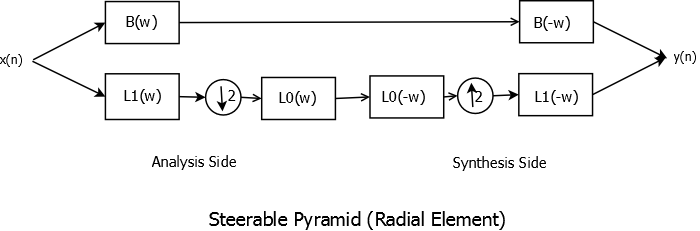
Single Stage Steerable Pyramid
\(B(\omega)\) is the band pass filter while \(L_{1}(\omega)\) and \(L_{0}(\omega)\) are the low pass filters. Band Pass filters are not subsampled in order to prevent aliasing while low pass filters are designed so that there is no aliasing (\( |L(\omega)| = 0, \forall \omega \geq \pi/2 \) ). Angular frequency computations depend on number of orientation bands needed. For example, if four orientation bands are used then the band pass filter is designed and rotated in four directions and each orientation \(\theta\) is essentially a weighted linear combination of four basis filters. A two-stage Pyramid implementation is shown below. Decomposition is carried out on the low pass branch. It is assumed that system response ( which is low pass) is actually \(L_{0}(\omega)\) which helps in designing low pass and band pass filters.

Two-Stage Steerable Pyramid
Steerable Pyramid Implementation
As an example of Steerable Pyramid implementation we will consider the pyramid shown below which was proposed by Simoncelli, et al. An image is pre-processed by filtering it along two channels - one high pass and the other low pass. The decomposition is done on the low pass image by further filtering it with oriented band pass filters. The number of band pass filters \(k\) is determined by the desired number of orientation bands. The cascaded pyramid structure is implemented by replacing \(\oplus\) in the low pass band by the entire structure contained within the dotted lines.
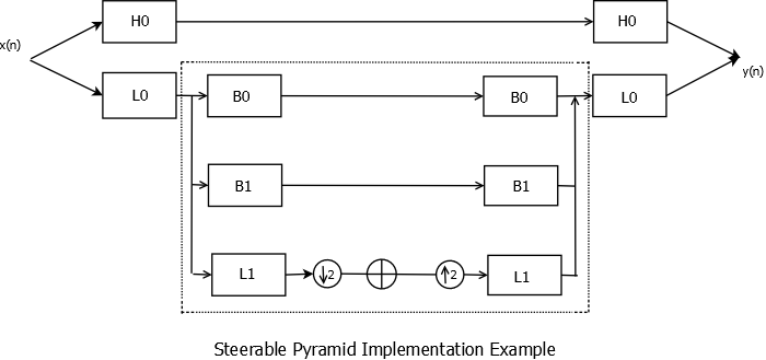
Steerable Pyramid Implementation
Filter Constraints
1. Perfect Reconstruction
a) Unity System Response Amplitude
\[ |L_{0}(\overline{\omega})|^{2}[|L_{1}(\overline{\omega})|^{2}+\sum_{n=0}^{k-1} |B_{n}(\overline{\omega})|^{2}]+|H_{0}(\overline{\omega})|^{2}=1 \]b) Cascaded Structure must preserve the prefect reconstruction condition and the low pass nature of the lower branch which gives us following equation
\[ |L_{1}(\overline{\omega/2})|^{2}[|L_{1}(\overline{\omega})|^{2}+\sum_{n=0}^{k-1} |B_{n}(\overline{\omega})|^{2}]=|L_{1}(\overline{\omega/2})|^{2} \]c) As mentioned earlier, low pass filters must be designed to prevent aliasing as we use subsampling in low pass branch.
\[ L_{0}(\overline{\omega})=0 \]for all \(|\omega| \gt \pi/2 \)
2. Orientation : Oriented Band Pass filters are given by
\[ B_{n}(\overline{\omega})=B(\overline{\omega})(-j cos(\theta-\theta_{n}))^{k-1} \]where \(\theta= \arg(\overline{\omega})\) , \(\theta_{n}= \frac{\pi n}{k}\) and \(n={0,1,...,k-1}\)
Filters Design
\(2D\) Filters for Steerable Pyramid can designed using techniques proposed by Karasaridis et al. and then by Castleman et al.\(L_{1}(\overline{\omega})\) is designed as a \(1D\) raised cosine filter. We then choose \(L_{0}(\overline{\omega})=L_{1}(\overline{\omega/2})\) and band pass filters are obtained using perfect reconstruction and angular constraints. These filters are converted to \(2D\) filters using McClellan Frequency Transformation outlined in Jae Lim's book. The chosen filters are all \(17 X 17 \) filters.
Steerable Pyramid for \(k=2\) Orientations
As can be seen from the Steerable Pyramid figure we need \(5\) filters to implement \(k=2\) orientation pyramid. The first two filters \(L_{0}\) and \(H_{0}\) are shown below. These two are also known as pre-processing filters(or post-processing filters at the reconstruction stage).
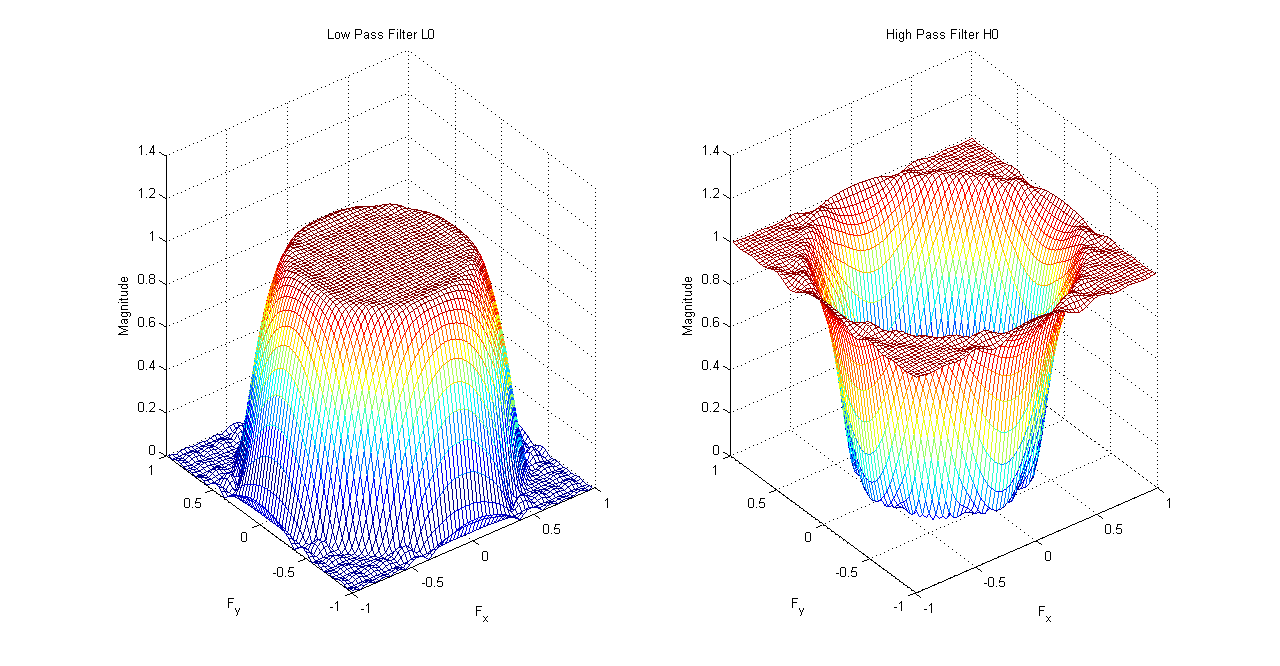
Steerable Pyramid Pre-Processing Filters \(L_{0}\) and \(H_{0}\)
The next set of filters are known also known as Iterated Filters as they are part of the cascaded stage of the Pyramid. We add \(N\) cascades for \(N\) level of decomposition. \(N=3\) is used in this example. The three filters are the low pass filter \(L_{1}\) and two oriented band pass filters \(B_{0}\) and \(B_{1}\).
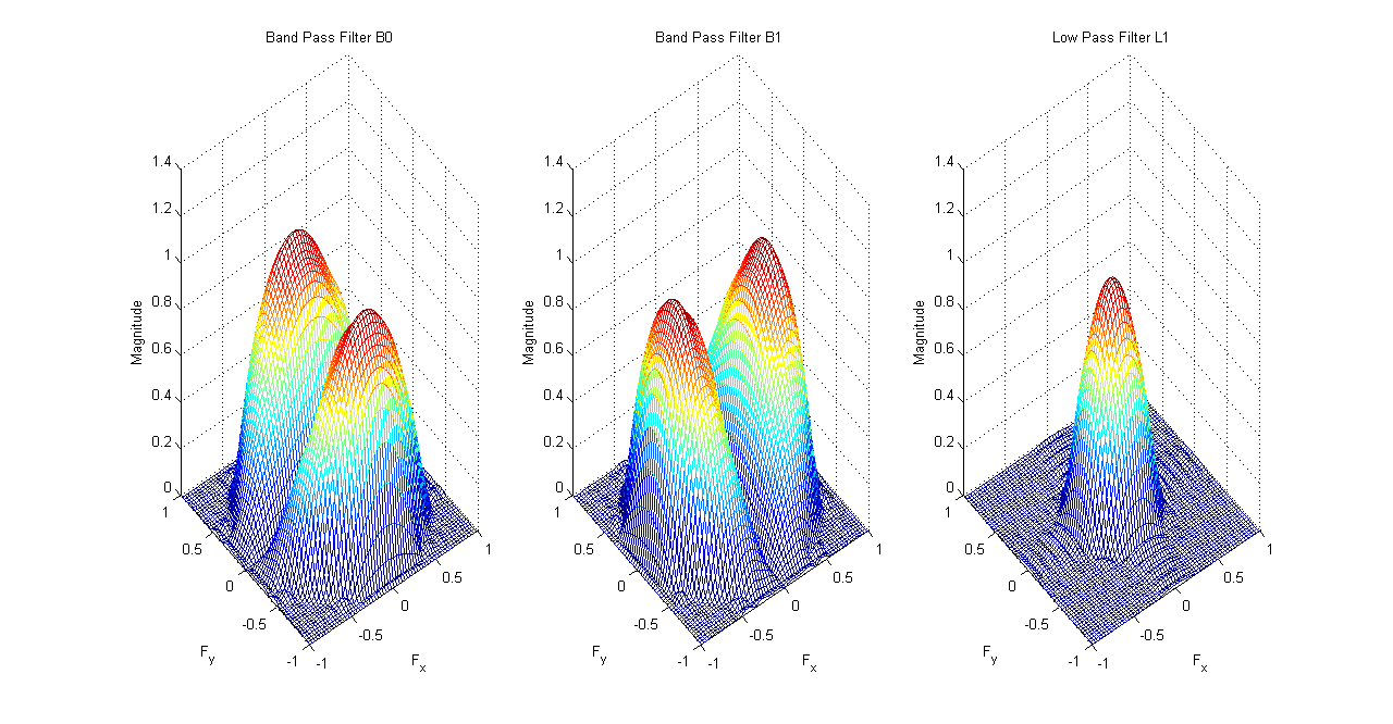
Steerable Pyramid Iterated Filters \(B_{0}\), \(B_{1}\) and \(L_{1}\)
This pyramid is used to decompose ``Zoneplate'' image at three scales. It can be seen that the images at all three scales are oriented in two different directions.
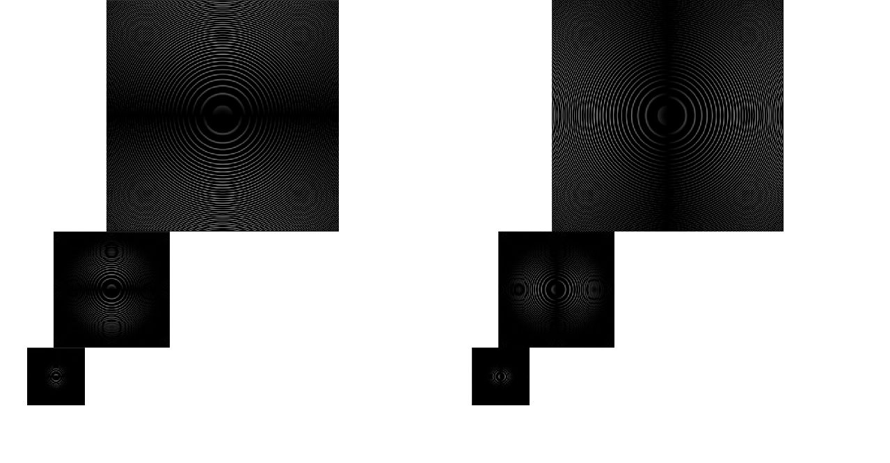
\(3\) Level \(k=2\) Oriented Decomposition of Zoneplate Image
Steerable Pyramid for \(k=3\) Orientations
The only difference between \(k=2\) and \(k=3\) or ,indeed, any other value of \(k\) is that we have to design \(k\) different abnd pass filters alongside two low pass and one high pass filters. Pre-processing and post-processing filters \(L_{0}\) and \(H_{0}\) filters are designed the same way and are shown below.
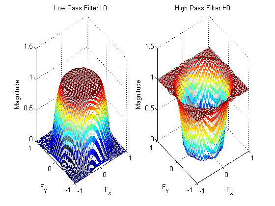
Steerable Pyramid Pre-Processing Filters \(L_{0}\) and \(H_{0}\)
As mentioned earlier, we will have to design three oriented band pass filters in this case. These three filters along with the iterated low pass filter \(L_{0}\) are shown in the following figure
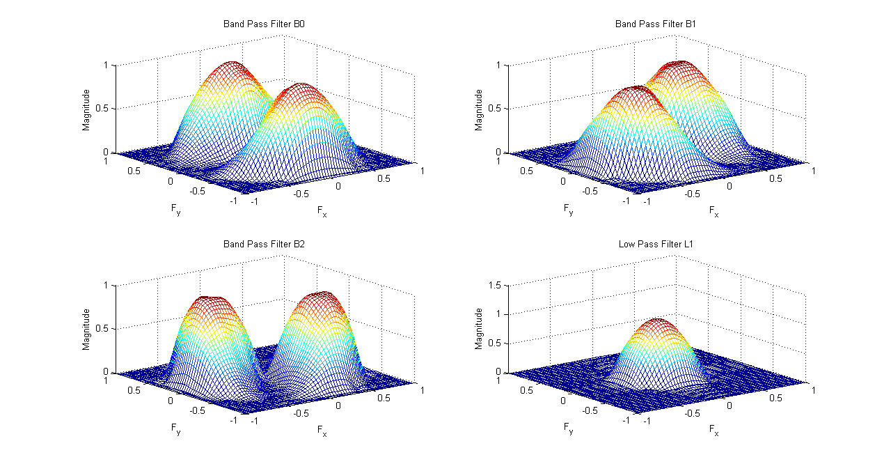
Steerable Pyramid Iterated Filters \(B_{0}\), \(B_{1}\), \(B_{2}\) and \(L_{1}\)
This Steerable Pyramid is used to decompose ``Zoneplate'' image at three scales. It can be seen that the images at all three scales are oriented in three different directions.
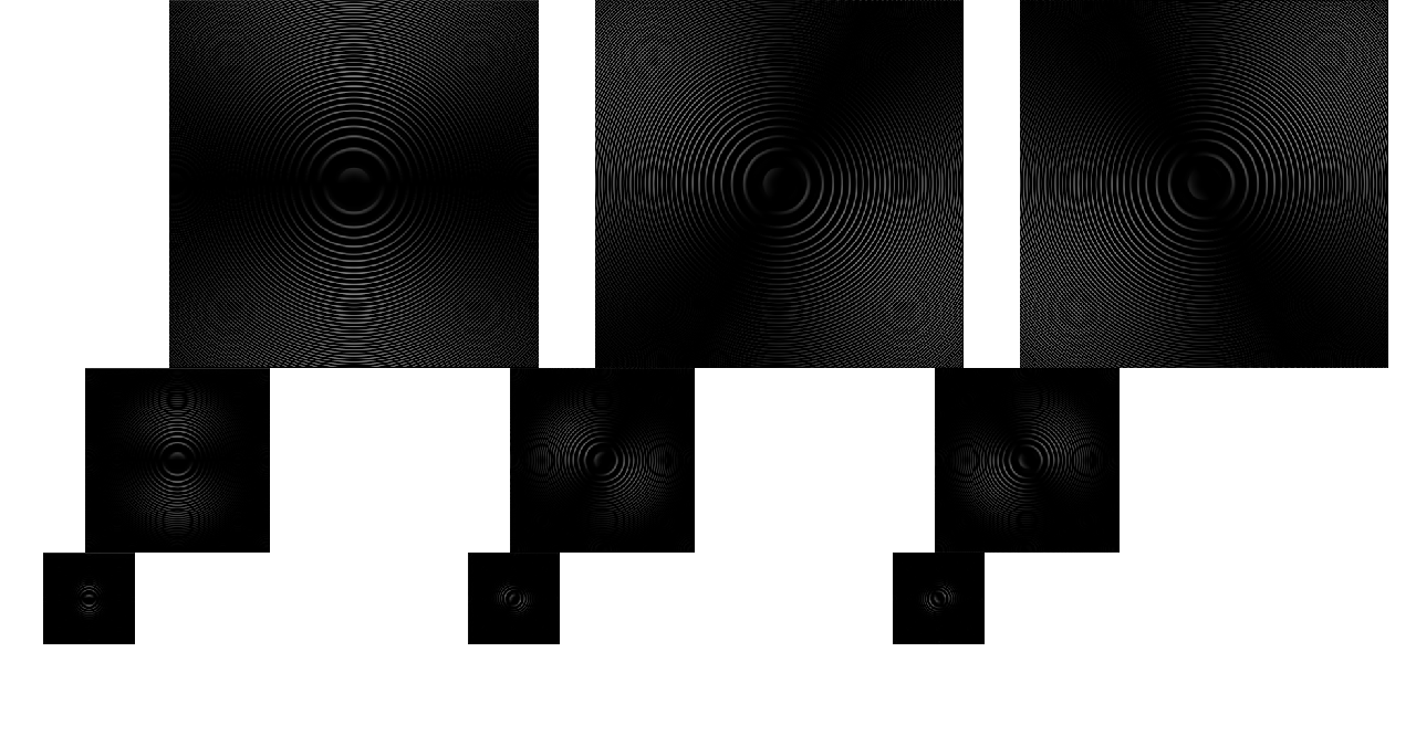
\(3\) Level \(k=3\) Oriented Decomposition of Zoneplate Image