
Two Dimensional Wavelet transform
Two dimensional wavelets and filter banks are used extensively in image processing and compression applications. It is easy to extend 1D ideas to 2D. We'll start with dilation equations.
\[ \phi(x_{1},x_{2})=\sum_{n_{1}}\sum_{n_{2}} h_{0}(n_{1},n_{2})\phi(2x_{1}-n_{1},2x_{2}-n_{2}) \]where \(h_{0}\) is a 2D low pass filter while \(\phi\) is a 2D scaling function. As is obvious , we are interested in \(L^{2}(R^{2})\) spaces and in \(L^{2}(R^{2})\) space filter implementations we have two options. Either we can design 2D filters or we can use 2 1D filters to create one 2D filter. Wavelets bases obtained from former are called nonseparable wavelet bases while latter yields separable bases.
Let \(h\) be a 1D low pass filter while \(g\) be the corresponding high pass filter. The scaling dilation equation can be written as
\[ \phi(x_{1},x_{2})=\sum_{n_{1}}\sum_{n_{2}} h(n_{1})h(n_{2})\phi(2x_{1}-n_{1},2x_{2}-n_{2}) \]We'll have three, not one, wavelet dilation equations and three mother wavelets.
\[ \psi_{hg}(x_{1},x_{2})=\sum_{n_{1}}\sum_{n_{2}} h(n_{1})g(n_{2})\phi(2x_{1}-n_{1},2x_{2}-n_{2}) \] \[ \psi_{gh}(x_{1},x_{2})=\sum_{n_{1}}\sum_{n_{2}} g(n_{1})h(n_{2})\phi(2x_{1}-n_{1},2x_{2}-n_{2}) \] \[ \psi_{gg}(x_{1},x_{2})=\sum_{n_{1}}\sum_{n_{2}} g(n_{1})g(n_{2})\phi(2x_{1}-n_{1},2x_{2}-n_{2}) \]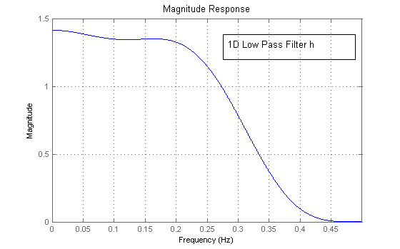
1D Low Pass Filter h
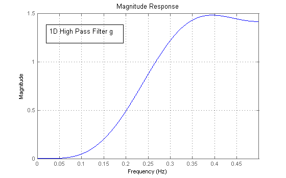
1D High Pass Filter g
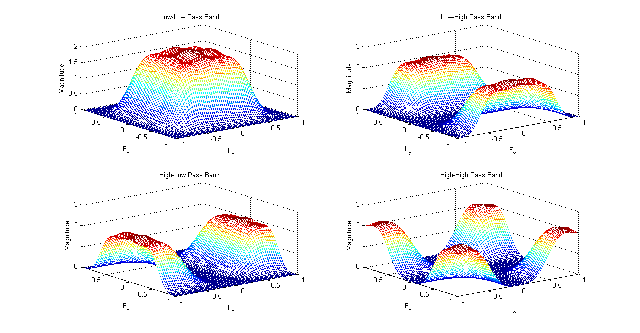
2D Filters obtained from h and g
This idea will be made clearer shortly.
Two-Dimensional Separable Multiresolutions
All 1D ideas can be directly applied to 2D separable Multiresolution case. The spaces are usually represented as \(V_{j}^{2}\) and \(W_{j}^{2}\) where \(V_{j}^{2}\) is a tensor product of two 1D spaces.
\[ V_{j}^{2}=V_{j}\otimes V_{j} \] while nesting is similar to 1D case as well \[ V_{j+1}^{2}=V_{j}^{2}\oplus W_{j}^{2} \]The two dimensional wavelets and scaling functions can also be represented in terms of their 1D counterparts.Consider, \(L^{2}(R^{2})\) space with 1D scaling functions \(\phi(x_{1})\) and \(\phi(x_{2})\) corresponding to each dimension.The wavelets are given by \(\psi(x_{1})\) and \(\psi(x_{2})\). We are using a one-to-one correspondence with filters \(h\) and \(g\) here with \(\phi\) being associated with low pass filter and \(\psi\) with high pass filter. Corresponding to four different filter configurations seen above, we have one scaling function and three wavelets.
\[ \phi(x_{1},x_{2})=\phi(x_{1})\phi(x_{2}) \] \[ \psi^{1}(x_{1},x_{2})=\phi(x_{1})\psi(x_{2}) \] \[ \psi^{2}(x_{1},x_{2})=\psi(x_{1})\phi(x_{2}) \] \[ \psi^{3}(x_{1},x_{2})=\psi(x_{1})\psi(x_{2}) \]If \(\phi\) and \(\psi\) are orthonormal basis functions in a MRA spanned by \(V_{j}\) and \(W_{j}\) then the corresponding 2D space is also orthonormal. The three wavelets \(\psi_{j,n}^{1}\), \(\psi_{j,n}^{2}\) and \(\psi_{j,n}^{3}\) form an orthonormal basis. Corresponding to these three wavelets we have three wavelet spaces that are given by
\[ W_{j}^{2}=(V_{j}\otimes W_{j}) \oplus (W_{j}\otimes V_{j}) \oplus (W_{j}\otimes W_{j}) \]We can extend orthonormal MRA idea to biorthogonal MRA which is actually a set of two MRAs- one ``normal'' MRA and other ``tilde'' MRA. Common notation is to denote analysis filter banks as ``tilde'' MRA.
2D DWT Algorithm
2D DWT algorithm is developed the same way as the 1D algorithm. Let \(S_{j,k}\) and \(W_{j,k}^{k}\) be scaling and wavelet coefficients at scale \(j\) for a given signal \(f(t)\) where \(k=1,2,3\).We'll be working with separable orthonormal filters so 2D filters can be expressed as a product between low pass filter \(h\) and high pass filter \(g\). Proceeding as before, the coefficients at scale \(j\) can be obtained from coefficients at scale \(j+1\)
\[ S_{j,v} = 2^\frac{1}{2}\sum_{k} hh(l-2v) S_{j+1,l} \] \[ W_{j,v}^{1} = 2^\frac{1}{2}\sum_{k} hg(l-2v) S_{j+1,l} \] \[ W_{j,v}^{2} = 2^\frac{1}{2}\sum_{k} gh(l-2v) S_{j+1,l} \] \[ W_{j,v}^{3} = 2^\frac{1}{2}\sum_{k} gg(l-2v) S_{j+1,l} \]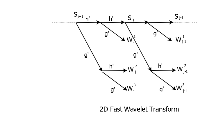
2D Fast Wavelet Transform
Looking at 2D Fast Wavelet transform diagram, 2D filters are developed using two 1D filters in each branch. Just as in 1D case, these filters are time-reversed and decimated by 2. To implement this filter bank, we use two-stage filter banks. In the first stage, rows of two dimensional signal are convolved with \(h\),\(g\) filters and then we downsample columns by \(2\) (eg., we keep only even indexed columns). In the next stage, columns are convolved with the filters \(h\),\(g\) and we keep only even indexed rows. In other words, a \(N*N\) image is transformed into two \(N*(N/2)\) images after first stage and four \((N/2)*(N/2)\) images after the second stage.

2D DWT Filter Bank Implementation
Following is a \(1\)-level and \(2\)-level decomposition of ``Lena'' image using the 2D filter bank.
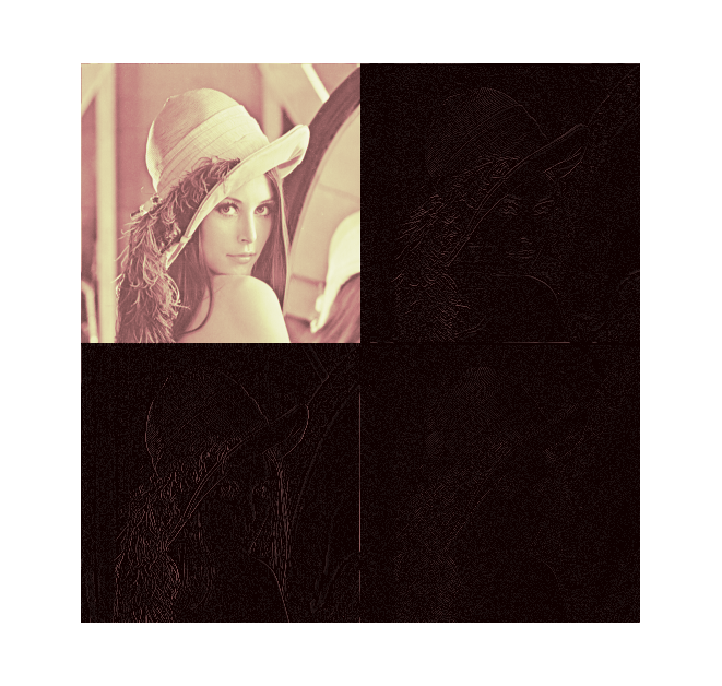
1-level Decomposition of Lena Image
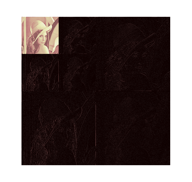
2-level Decomposition of Lena Image
To understand the decomposition process, we need to look at it through the wavelet filter banks and vanishing moment approach. If the wavelet high pass filter has \(N\) zeros at \(\omega=0\) then it will annihilate any polynomial signal with degree less than \(N\). A \(2D\) separable filter bank is essentially a two stage filter bank which performs operations in the horizontal direction first (rows) and then the vertical direction(columns). For Lo-Hi band, the high pass filtering occurs in the vertical direction and hence all vertical direction polynomials of degree \(N-1\) are annihilated and it accentuates the horizontal direction edges. For Hi-Lo band the horizontal direction is high pass filtered first which removes horizontal edges and vertical edges are accentuated after the low pass filtering in stage II. For Hi-Hi band case both horizontal and vertical directions are annihilated so edges that are at an angle to the horizontal and vertical will have large coefficients with their maxima being reached at diagonals. However,it should be kept in mins that this configuration isn't very helpful for edges that are at an angle. Directional , nonseparable filter banks usually give better results for images with non-horizontal and non-vertical edges with increased complexity being the trade-off.