Image processing
Image Denoising
\(2D\) Discrete Wavelet works similarly to \(1D\) transform and \(1D\) denoising principles can be used to denoise \(2D\) signals.\(2D\) decomposition transforms an image into \(4\) subimages, each a quarter size of the original, at each level.Of these \(subimages\), three are detail images and one is the approximation image. Denoising methods focus on these three detail images as they are the ones that contain high frequencies in at least one direction. A generic denoising algorithm is given as
- 1. Calculate DWT of a noisy image.
- 2. Use thresholding in all the detail images to get rid of high spatial-frequency components.
- 3. Take Inverse DWT of thresholded signal.
There are different thresholding algorithms involving different trade-offs as a strict threshold results in loss of data while a more lax threshold leaves noise in the image.
There are a number of algorithms( see references) that are used to denoise images. One of those method is Visushrink , which isn't a really efficient method but is good to illustrate the denoising process as it uses global thresholding. The threshold is chosen to be \(T=\sigma \sqrt{2 \log M}\) where \(M\) is the number of pixels in the detail subimages.Hard thresholding is pretty straightforward as all coefficients below the chosen threshold are set to zero and results in a relatively poor performance as too many coefficients are set to zero.

Noisy lena Image

Denoised Image using hard thresholding
Soft thresholding function is given by \(f_{s}(y,T)=sign(y) max(|y|-T,0)\).

Denoised Image using soft thresholding
Soft thresholding gives better results. For more and better algorithms, including those utilizing local thresholds, see references.
Wavelet Edge Detection
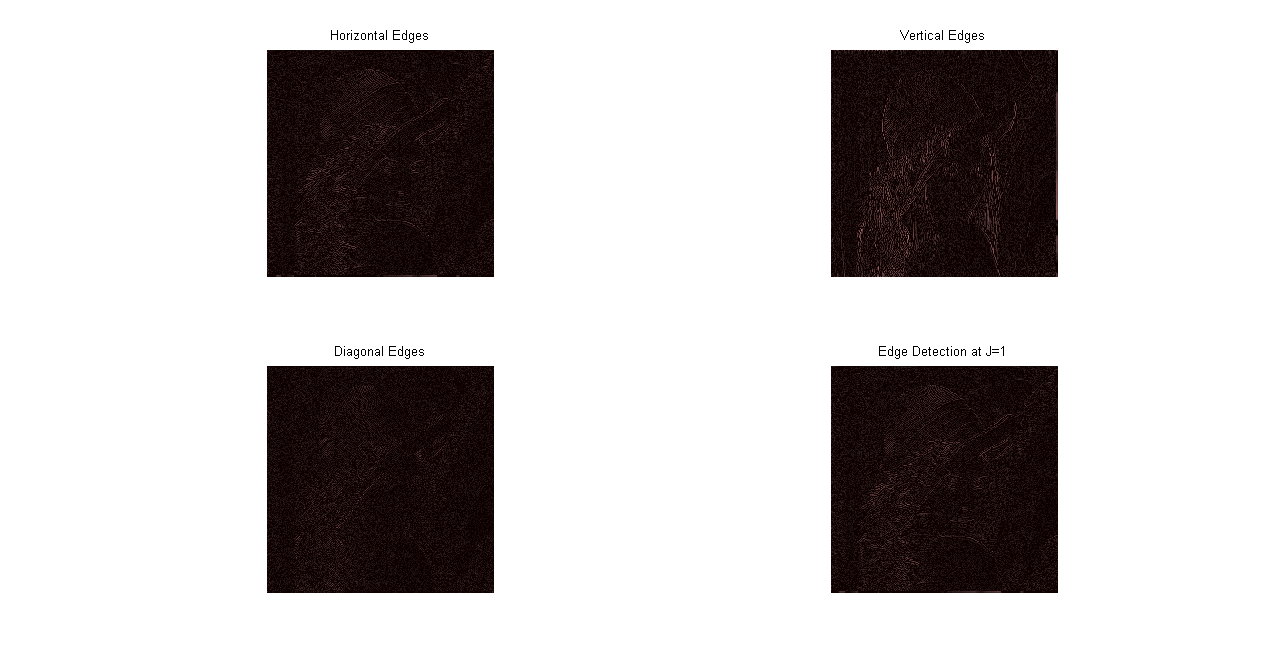
Wavelets perform well as singularity/discontinuity detector in one dimension so it makes sense to extend the same ideas to two dimensions and edge detection. We know that one level of separable wavelet decomposition yields four subimages and three of these four subimages correspond to horizontal , vertical and diagonal edges. For a straightforward wavelet edge detector implementation, all three detail subimages can be linearly combined to give an edge detector at a given scale as shown in the figure below. The edge detector is implemented using ``Db4'' orthogonal wavelets and it isn't thresholded. Thresholding can be applied to yield better results but it is obvious from the figure that this is not an optimal solution. It is too noisy and some true edges are missed while false edges are being detected. One of the big issue of using high frequency response is that it contains noise and most edge detectors used in computer vision and image processing literature use smoothing gaussian filters to get rid of noise. It has been suggested that applying Gaussian pre-processing to standard wavelet transforms will yield better results. A better approach is to use wavelets that are derived from these isotropic smoothing functions like Gaussians and splines.

Edge Detection at Scale J=1
Mallat's Multiscale Edge Detector
Let \(\theta(x)\) be a smoothing function,ie. \( \int_{-\infty}^{\infty} \theta(x) dx=1\), then the wavelet \(\psi(x)\) can be defined as
\[ \psi(x)=\frac{d\theta}{dx} \]In his 1992 paper, Mallat designed wavelets and filters using a smoothing function with Fourier Transform
\[ \theta(\omega)= \left[\frac{\sin(\omega/4)}{\omega/4}\right]^{(2n+2)} \]The scaling and wavelet functions are given by
\[ \phi(x)=\left[\frac{\sin(\omega/2)}{\omega/2}\right]^{(2n+1)} \] \[ \psi(x)=i\omega \left[\frac{\sin(\omega/4)}{\omega/4}\right]^{(2n+2)} \]Filters are designed for \(n=1\) in the example below. For 2d implementation, we use two smoothing functions \(\theta_{1}(x)\) and \(\theta_{2}(x)\) and we assume that they are approximately equal. The two wavelets are then given by
\[ \psi_{1}(x,y)=\frac{d\theta_{1}(x,y)}{dx} \] \[ \psi_{2}(x,y)=\frac{d\theta_{2}(x,y)}{dy} \]They can be further defined by as separable computations of one dimensional functions.
\[ \psi_{1}(x,y)=2\psi(x)\phi(2y) \] \[ \psi_{2}(x,y)=2\psi(y)\phi(2x) \]Each signal \(s_{2^{j+1}}^{d}(f)\) is decomposed into three signals - a low pass smoothed signal \(s_{2^{j}}^{d}(f)\) and two high pass components that correspond to horizontal and vertical edges if the input signal is an image, namely \(w_{2^{j}}^{1,d}(f)\) and \(w_{2^{j}}^{2,d}(f)\). The modulus \(M\) of the signal is computed as
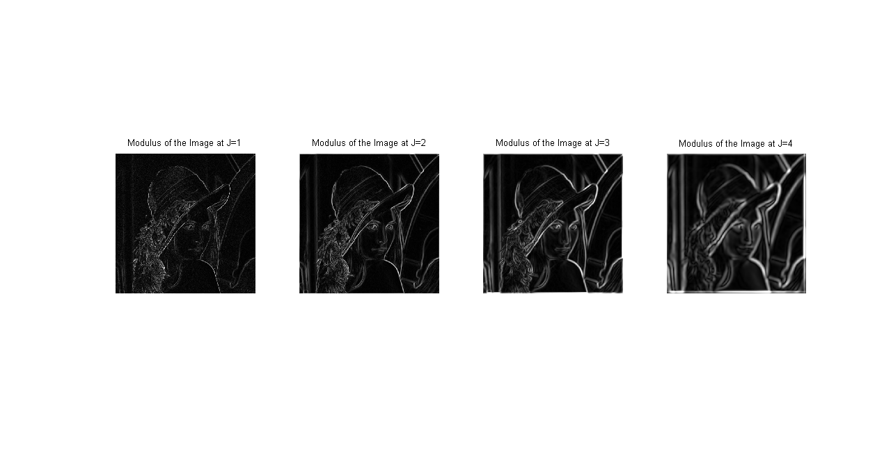
\[ M_{2^{j}}(f)=\sqrt{ |w_{2^{j}}^{1,d}(f)|^{2}+|w_{2^{j}}^{2,d}(f)|^{2}} \]at each point \((x,y)\). An example of this Multiscale edge detector is shown below. The treatment of edge detector on this page is incomplete as of now so please see references for proofs and methods to compute Wavelet Transform Modulus Maxima.

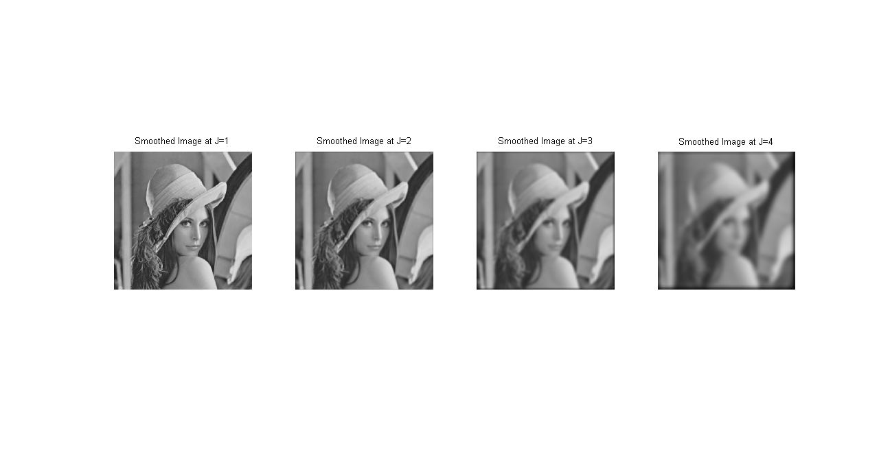
Lena Image at J=1,2,3,4

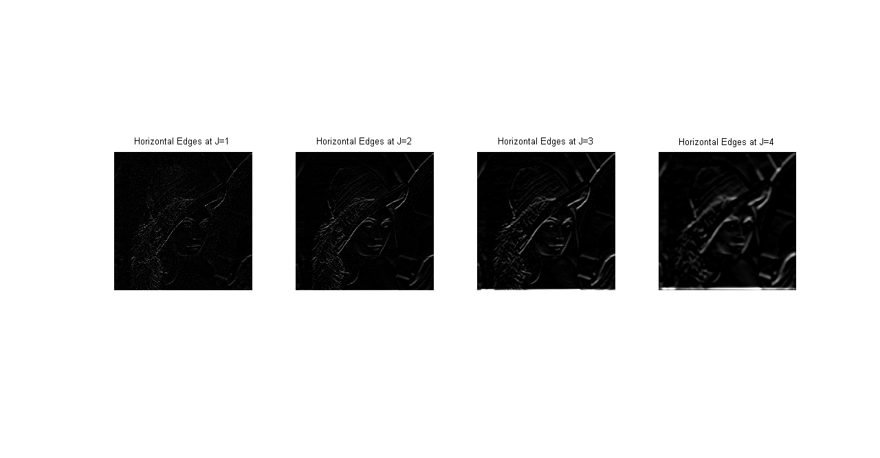
Horizontal Edges at J=1,2,3,4

Vertical Edges at J=1,2,3,4

Image Modulus at J=1,2,3,4
