
Multiresolution Analysis
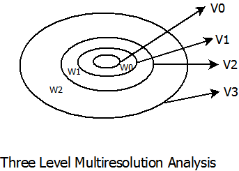
Mother Wavelet \(\psi(t)\) is an orthonormal wavelet if its translates and dilates are orthonormal under the inner product. \[ \lt\psi_{j,k},\psi_{l,m}\gt=\int_{-\infty}^{\infty}\psi_{j,k}(t)\psi_{l,m}^\ast(t)dt = \delta_{j,l}\delta_{k,m} \] where \(j,k,l,m\in\)\(Z\) and \(\delta\) is the Kronecker delta function. Such a wavelet system is self-dual,ie., for a given function \(f(x)\)The idea of Multiresolution is to decompose a signal \(f(t)\in L^2(R)\) such that orthogonal projections of \(f(t)\) given by \(f_j\) ``live'' in the space \(V_j\).\(V_j\) and \(W_j\) are complementary subspaces with \(W_j\) being the difference between \(V_j\) and \(V_{j+1}\).
\[ V_{j+1}=V_j\oplus W_j \]Multiresolution approximation, as defined by Mallat and Meyer, has the following properties.
1. \(V_{j} \subset V_{j+1}\) A function in subspace \(j\) is in all the finer subspaces. In other words, if we know a signal \(f_{j}(t)\) at subspace \(V_{j}\), we can obtain ts coarse approximation using MRA. Think of a signal being decomposed using an iterated chain of complementary low pass and high pass filters. At every step we obtain a low pass and high pass version of the signal from the previous step. However, the low pass signal in step two is contained in the signal from the step one.
2. \(f(t) \in V_{0} \Leftrightarrow f(t-k) \in V_{0}\) This is the translation (shift) invariant property of the subspace. A signal in a given subspace , if translated by \( k \in Z \) is still in that subspace. This property is valid for all subspaces.
3. \(f(t) \in V_{j} \Leftrightarrow f(2t) \in V_{j+1}\) This is the scale invariant property of the Multiresolution analysis. In frequency domain terms, \( f(2t) \) contains \(2X\) highest frequency compared to that contained in \(f(t)\). Using iterated filter bank example with a low pass filter that halves the frequencies in every step, it becomes clear that moving back one step in each step of the filter chain doubles the highest frequency content.
Multiresolution Analysis
4. \(\bigcap_{j \rightarrow {-\infty}} V_{j}=\{0\}\) As we move to lower subspaces, the space occupied by \(V_{j}\) shrinks until it becomes nearly zero.
5.\(\bigcup_{j \rightarrow {\infty}} V_{j}=L^2(R)\) Union of all subspaces as \(j \rightarrow {\infty}\) encompasses the whole \(L^2(R)\) space.
Dilation Equation
Let \(f_{0}(t)\) and \(f_{1}(t)\) be the projections of signal \(f(t)\) associated with subspaces \(V_{0}\) and \( V_{1}\) respectively. The difference of these two projections ``lives'' in the complementary Wavelet space \(W_{0}\).
According to 1, \(V_{0} \subset V_{1}\). Let \(\phi(t)\) and \(\psi(t)\) be the scaling and wavelet functions associated with subspaces \(V_{0}\) and \(W_{0}\). It follows from 1 that \(\phi(t)\) is contained in \(V_{1}\) and can be expressed in terms of \(\phi(2t)\).
\[ \phi(t)=2^\frac{1}{2}\sum_{k} h(k)\phi(2t-k) \]The term \(2^\frac{1}{2}\) comes from the definition of basis function at scale \(j=1\). The equation above is known as the dilation equation and forms the bridge between wavelets and filterbanks. \(h(k)\) corresponds to the low pass filter that is associated with the scaling function. If \(g(k)\) is the complementary high pass filter in this orthogonal filterbank then the Wavelet equation can be expressed as
\[ \psi(t)=2^\frac{1}{2}\sum_{k} g(k)\phi(2t-k) \]The wavelet equation written above follows from the fact that \(W_{0}\) also nests inside \(V_{1}\) and can be obtained by using the similar process as used in the scaling function case.
Wavelet Transform Algorithm
Again from 1, \(\psi_{j,k}(t)\) and \(\phi_{j,k}(t)\) can be represented by \(\phi_{j+1,k(t)}\). Let \(S_{j,k}\) and \(W_{j,k}\) be scaling and wavelet coefficients at scale \(j\) for a given signal \(f(t)\).
\[ S_{j,k}=\int_{-\infty}^{\infty} f(t) \phi_{j,k}(t)dt \] \[ W_{j,k}=\int_{-\infty}^{\infty} f(t) \psi_{j,k}(t)dt \]Using MRA properties, \[ \sum S_{j+1,k} \phi_{j+1,k}(t) = \sum W_{j,k} \psi_{j,k}(t) + \sum S_{j,k} \phi_{j,k}(t) \] as signal projection \( f_{j+1}(t)=f_{j}(t)+\Delta f_{j}(t) \) where \(\Delta f_{j}(t) \) is the signal projection in the wavelet space. We shift dilation and wavelet equations by v and generalize to scale j.
\[ \phi(2^{j}t-v)=2^\frac{1}{2}\sum_{k} h(k)\phi(2^{j+1}t-2v-k) \] \[ \psi(2^{j}t-v)=2^\frac{1}{2}\sum_{k} g(k)\phi(2^{j+1}t-2v-k) \]Substituting \(l=2v+k\) and integrating by multiplying both equations by \(f(t)\) gives
\[ \int_{-\infty}^{\infty} f(t) \phi_{j,v}dt=2^\frac{1}{2}\sum_{k} h(l-2v) \int_{-\infty}^{\infty} f(t) \phi_{j+1,l}(t) dt \] \[ \int_{-\infty}^{\infty} f(t) \psi_{j,v}dt=2^\frac{1}{2}\sum_{k} g(l-2v) \int_{-\infty}^{\infty} f(t) \phi_{j+1,l}(t) dt \]Using values of \(S_{j,k}\) and \(W_{j,k}\) from above yields
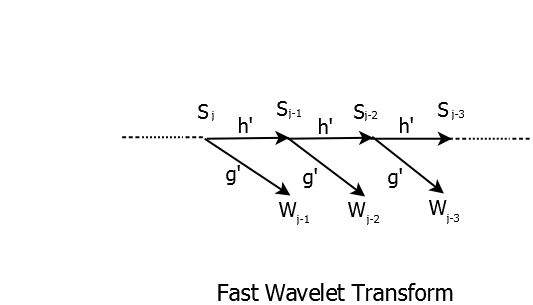
\[ S_{j,v} = 2^\frac{1}{2}\sum_{k} h(l-2v) S_{j+1,l} \] \[ W_{j,v} = 2^\frac{1}{2}\sum_{k} g(l-2v) S_{j+1,l} \]where \(h(l-2v)\) and \(g(l-2v)\) can be thought of as time-reversed and decimated by 2 low pass and high pass filters. This is the fast wavelet transform algorithm.
The Inverse Fast Wavelet transform is simply inverse of the FWT and can be easily shown using same equations. More on Filterbanks and Wavelets will be covered in next chapter.