Non-Linear Approximation

In data compression applications, a good approximation error rate decay is crucial and it makes sense to utilize wavelet property of returning large coefficients at discontinuities and signal fluctuations. For an orthonormal basis \(e_{k}\), the approximation error is given by

In linear case, we choose first \(M\) coefficients ,eg. in Fourier domain we go with lowest \(M/2\) positive and negative frequencies and in wavelet domain we choose first \(M\) coefficients starting with the coarsest scale. In Nonlinear case,we go with \(M\) largest coefficients by choosing the \(M\) largest inner products. So instead of dividing the coefficient space linearly, we do an nonlinear division by allocating coefficients in two sets denoted by ,say, \(I_{m}\) which contains the \(M\) largest coefficients and a set which contains all other coefficients.

The best nonlinear approximation is ,therefore, given by

for an orthonormal basis. The approximation error is given as before

Non-Linear Approximation Error Decay

Let us consider Fourier Transform first. If the function is smooth, Fourier transforms do a good job as most energy is concentrated in the lower frequencies and there is not much difference in using Linear and Non-linear Fourier approximation. If the function is piece-wise smooth, ie. it has discontinuities at points \(t_{k}\), fourier approximation does not give us appreciably better results as largest coefficients are clustered at the lowest frequencies that we pick in linear case anyway.It has been proven that approximation error rate decays as \(1/M\) in Fourier case.

Wavelets return large coefficients value at singularities, discontinuities etc. at every scale. If we are using linear approximation, we start with coarse scales and move to the finer scales but as is obvious quite a few large coefficients are ignored using this method. Let us suppose that there are \(M\) large coefficients distributed over \(M\) scales. If we are using non-linear approximation we can conceivably pick out all of these \(M\) coefficients instead of picking \(M\) coefficients across only \(J < M\) scales. The amplitude of wavelet coefficient is proportional to \(2^{-j/2}\) at scale \(j\). So if we stop at scale \(J < M\) using linear approximation, the last coefficients picked are of the order \(2^{-J/2}\) while the largest coefficient not selected has an amplitude in the range of \(2^{-(J+1)/2}\). However, if we are using non-linear approximation, the largest coefficient not picked will have the order \(2^{-(M+1)/2}\) so we see that in non-linear case , the error is decaying exponentially.

This can be demonstrated in Matlab using the following script

function f=nlapprox

% Linear Fourier and Wavelet Approximations using 100 
%coefficients out of 256
f = load_signal('Piece-Regular', 256); % Using this Wavelab
% function to generate a piecewise signal
x=f';% Preparing signal for wt.m
% Fourier Nonlinear Aproximation using 100 coefficients
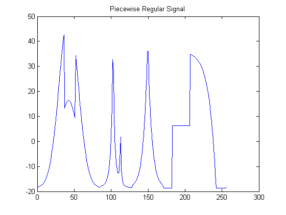
figure(1);plot(x),title('Piecewise Regular Signal');
yf=fft(x);
yf_shift=fftshift(yf);
% plot(abs(yf_shift));
% Signal reconstruction using all coeffiecients
% oup_f=ifft(yf);
% figure(2)
% plot(real(oup_f));

% Signal Reconstruction using n=100 coefficients

% Nonlinear Fourier Approximation
n=100;
N=length(yf_shift);
tf=findthresh(yf_shift,n);
yf_shift(abs(yf_shift)\< tf)=0;%Remove "\"
yf_appx=fftshift(yf_shift);
oup_f=ifft(yf_appx);
figure(2)
plot(real(oup_f));
title(' Nonlinear Fourier Approximation 100/256 coeffs');

% Linear Wavelet Approximation

% Signal is decomposed to level-4 and signal 
% is thresholded to choose 100 coefficients
% Using Db2 wavelets
[lp,hp,lp2,hp2]=wfilters('db2');
J=4;
[cA,cD,dcoeff]=wt_test(x,J,lp,hp);

% Choosing 100 coefficients
% All 256 coefficients are processed to find the 
%threshold and the largest 100 coefficients are chosen
 % while those below the thresold are set to zero.
coeff2=[cA,dcoeff(4,1:16),dcoeff(3,1:32),....
                    dcoeff(2,1:64),dcoeff(1,1:128)];
tw=findthresh(coeff2,n);
coeff2(abs(coeff2)\< tw)=0;%Remove "\"
cA=coeff2(1:16);
dcoeff(4,1:16)=coeff2(16+1:2*16);
dcoeff(3,1:32)=coeff2(32+1:2*32);
dcoeff(2,1:64)=coeff2(64+1:2*64);
dcoeff(1,:)=coeff2(128+1:2*128);
figure(3)
yw=iwt_test(cA,dcoeff,J,lp2,hp2);
plot(yw),title('Nonlinear Wavelet Approximtion 100/256 coeffs');
 
	

N=256 Piecewise Regular Signal

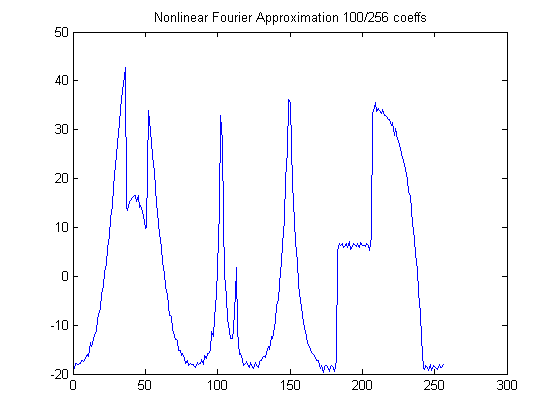
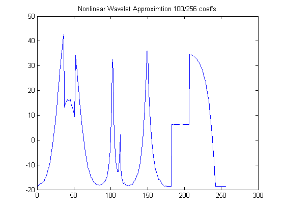
As can be seen from the program , a threshold is chosen depending on the number of approximation coefficients and all coefficients that fall below this threshold are set to zero. We calculate Inverse FFT and Inverse DWT based on these new values of coefficients. While Nonlinear Fourier Approximation doesn't show much improvement over its linear counterpart but ,as expected Nonlinear Wavelet approximation shows dramatic improvement over linear Wavelet Approximation.

100 coefficients Nonlinear Fourier Approximation

100 coefficients Nonlinear Wavelet Approximation