MultiWavelets

MultiWavelet Dilation Equation

Multiwavelet Dilation( Refinement) Equation is given by

\[ \overline{\phi}(x)=\sqrt{M} \sum_{k} H_{k} \overline{\phi}(Mx-k) \] \(k \in Z\)

where \(\overline{\phi}(x)\) is a \(r X 1\) vector given by

\[ \overline{\phi}(x)=\begin{bmatrix} \phi_{1}(x) \\ \phi_{2} (x) \\ . \\ . \\ \phi_{r} (x) \end{bmatrix} \]

and \(H_{k}\) is a \(rXr\) matrix. Additionally, \(r\) is known as Multiplicity and \(M\) is known as Dilation Factor. Scalar wavelets can be seen as a special case of Mutiwavelets with \(M=2\) and \(r=1\).

Orthogonality Condition

The scaling vector \(\overline{\phi}(x)\) is orthogonal if

\[ \lt \overline{\phi}(x),\overline{\phi}(x-k) \gt = \int \overline{\phi}(x) \overline{\phi}^{*}(x-k) dx = \delta_{0,k} I \]

where \(I\) is a \(rXr\) identity matrix. Or, equivalently the orthogonality can be given in terms of \(H_{k}\) matrix

\[ \sum_{k} H_{k}H_{2l+k}^{T}=\delta_{0,l} I \]

The equation above can be proved by substituting dilation equation into the inner product equation.

DGHM Multiscaling Functions

Donovan, Geronimo, Hardin and Massopust proposed DGHM wavelets that are defined by the following recursion coefficients (\(H_{k} matrices\)

\[ H_{0}=\frac{1}{20 \sqrt{2}}\begin{bmatrix} 12 & 16 \sqrt{2} \\ -\sqrt{2} & -6 \end{bmatrix} \] \[ H_{1}=\frac{1}{20 \sqrt{2}}\begin{bmatrix} 12 & 0 \\ 9 \sqrt{2} & 20 \end{bmatrix} \] \[ H_{2}=\frac{1}{20 \sqrt{2}}\begin{bmatrix} 0 & 0 \\ 9 \sqrt{2} & -6 \end{bmatrix} \] \[ H_{3}=\frac{1}{20 \sqrt{2}}\begin{bmatrix} 0 & 0 \\ -\sqrt{2} & 0 \end{bmatrix} \]

DGHM Multiscaling functions are orthogonal as

\[ \sum_{k=0}^{3} H_{k}H_{2l+k}^{T}=\begin{bmatrix} 1 & 0 \\ 0 & 1 \end{bmatrix} \]

MultiWavelet Multiresolution Analysis

Orthogonal MultiWavelet MRA is identical to scalar wavelets MRA with following properties.

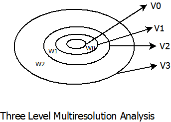
• 1. \(V_{j} \subset V_{j+1}\) A function in subspace \(j\) is in all the finer subspaces. In other words, if we know a signal \(f_{j}(x)\) at subspace \(V_{j}\), we can obtain ts coarse approximation using MRA. Think of a signal being decomposed using an iterated chain of complementary low pass and high pass filters. At every step we obtain a low pass and high pass version of the signal from the previous step. However, the low pass signal in step two is contained in the signal from the step one.


• 2. \(f(t) \in V_{0} \Leftrightarrow f(x-k) \in V_{0}\) This is the translation (shift) invariant property of the subspace. A signal in a given subspace , if translated by \( k \in Z \) is still in that subspace. This property is valid for all subspaces.


• 3. \(f(x) \in V_{j} \Leftrightarrow f(2x) \in V_{j+1}\) This is the scale invariant property of the Multiresolution analysis. In frequency domain terms, \( f(2t) \) contains \(2X\) highest frequency compared to that contained in \(f(t)\). Using iterated filter bank example with a low pass filter that halves the frequencies in every step, it becomes clear that moving back one step in each step of the filter chain doubles the highest frequency content.





MultiWavelet MRA

• 4. \(\bigcap_{j \rightarrow {-\infty}} V_{j}=\{0\}\) As we move to lower subspaces, the space occupied by \(V_{j}\) shrinks until it becomes nearly zero.


• 5.\(\bigcup_{j \rightarrow {\infty}} V_{j}=L^2(R)\) Union of all subspaces as \(j \rightarrow {\infty}\) encompasses the whole \(L^2(R)\) space.


• 6. Multiwavelets: We define functions \(\overline{\psi}^{s}(x)\) such that they are orthogonal to \(\overline{\phi}(x)\) and to each other where \(\overline{\psi}^{s} \in L^{2}\) and \(s=1,... , M-1\). Given \(k \in Z\) , \(\overline{\psi}^{s}(x-k)\) forms a stable basis of \(W_{0}\).

Since each \(\overline{\psi}^{s} \in V_{1}\) , it can be written as \[ \overline{\psi}^{s}(x)=\sqrt{M} \sum_{k} G^{s}_{k} \overline{\phi}(Mx-k) \]

The functions \(\overline{\psi}^{s}\) are called multiwavelet functions.

Orthonormality Conditions

\[ \sum G^{s}_{k} G^{t*}_{Ml+k}=\delta_{0l} \delta_{st} I \] \[ \sum G^{s}_{k} H^{*}_{Ml+k}= \sum H_{k} G^{s*}_{Ml+k}= 0 \]

Discrete MultiWavelet Transform

Let \(Q_{k}\) give detail at level \(k\) while \(P_{k}\) give approximation at that level.

\[ L^{2}= \oplus W_{n} \]

Therefore, a function \(f\) can be given as summation of details at all levels.

\[ f=\sum_{-\infty}^{\infty} Q_{k}f \] \[ L^{2}=V_{J} \oplus W_{j} \]

where \(j=J,..., \infty \) or,

\[ L^{2}= {\oplus}_{-\infty}^{\infty} W_{j} \]

as

\[ V_{n}={\oplus}_{k=-\infty}^{n-1} W_{k} \]

We observe that \(P_{l}f\) converges to \(f\) as \(l\rightarrow \infty\). Let \(P_{n}f\) be the projection of \(f\) in the space \(V_{n}\) and \(Q_{n}f\) be the projection of \(f\) in the space \(W_{n}\).

\[ V_{n}+W_{n}=V_{n+1} \]

or,

\[ V_{n}+W_{n}+W_{n+1}+...+W_{n+l}=V_{n+1+l} \]

Therefore, \(f=P_{n}f+\sum_{k=n}^{l} Q_{k}f\) for some \(l \gt n\) is the Discrete MultiWavelet Transform (DMWT) and it is identical to DWT.

\[ f=P_{n}f+\sum_{k=n}^{l} Q_{k}f \] \[ f=\sum_{j} a_{n,j} \overline{\phi}_{n,j} + \sum_{j} \sum_{s=1}^{M-1} d^{s}_{n,j} \overline{\psi}^{s}_{n,j} \]

where \(a_{n,j}\) and \(d^{s}_{n,j}\) are approximation and detail coefficients and identical to the DWT case.

Biorthogonal MRAs and MultiWavelets

As is the case with scalar wavelets, \(\overline{\phi}\) and \(\widetilde{\overline{\phi}}\) are scaling function vectors in the Synthesis and Analysis domain respectively.

Biorthogonality Condition

\[ \lt \overline{\phi}(x-k),\widetilde{\overline{\phi}}(x-l) \gt =\delta_{lk} I \]

In terms of low pass symbol

\[ \sum H_{k} \widetilde{H}_{k+Ml}^{*}=\delta_{0l} I \]

The two scaling equations are given by

\[ \overline{\phi}(x)=\sqrt{M} \sum_{k} H_{k} \overline{\phi}(Mx-k) \] \[ \widetilde{\overline{\phi}}(x)=\sqrt{M} \sum_{k} \widetilde{H}_{k} \widetilde{\overline{\phi}}(Mx-k) \]

Projections \(P_{n}f\) and \(\widetilde{P_{n}f}\) of a \(L^{2}\) function \(f\) onto \(V_{n}\) and \(\widetilde{V_{n}}\) are given as

\[ P_{n}f=\sum_{j} \widetilde{a_{n,j}} \overline{\phi}_{n,j} \]

and

\[ \widetilde{P_{n}}f=\sum_{j} a_{n,j} \widetilde{\overline{\phi}}_{n,j} \]

The approximation coefficients can be calculated as

\[ \widetilde{a_{n,j}} = \lt f,\widetilde{\overline{\phi}}_{n,j} \gt = \int f \widetilde{\overline{\phi}}_{n,j}^{*} dx \] \[ a_{n,j} = \lt f,\overline{\phi}_{n,j} \gt = \int f \overline{\phi}_{n,j}^{*} dx \]

Therefore,

\[ P_{n}f=\lt f,\widetilde{\overline{\phi}}_{n,j} \gt \overline{\phi}_{n,j} \]

and

\[ \widetilde{P_{n}}f=\lt f,\overline{\phi}_{n,j} \gt \widetilde{\overline{\phi}}_{n,j} \]

The projections \(Q_{n}f\) and \(\widetilde{Q_{n}}f\) are defined as

\[ Q_{n}f=P_{n+1}f-P+{n}f \] \[ \widetilde{Q_{n}}f=\widetilde{P_{n+1}}f-\widetilde{P_{n}}f \]

and the subspaces are non-orthogonal direct sums given by

\[ V_{n}+W_{n}=V_{n+1} \] \[ \widetilde{V}_{n}+\widetilde{W}_{n}=\widetilde{V}_{n+1} \]

Biorthogonality Conditions as applied to subspaces in multiwavelet case are same as in the scalar case.

\[ V_{n} \bot \widetilde{V}_{n} \] \[ V_{n} \bot \widetilde{W}_{n} \] \[ W_{n} \bot \widetilde{V}_{n} \]

and

\[ W_{n} \bot \widetilde{W}_{n} \] if \(k \neq n\)

Discrete MultiWavelet Transform (DWMT) in this case is same as that in scalar biorthogonal DWT case. Biorthogonalty conditions in terms of low pass and high pass symbols are given as

\[ \sum H_{k} \widetilde{H}_{k+Ml}^{*}=\delta_{0l} I \] \[ \sum G^{s}_{k} \widetilde{G}^{t*}_{Ml+k}=\delta_{0l} \delta_{st} I \] \[ \sum G^{s}_{k} \widetilde{H}^{*}_{Ml+k}= \sum H_{k} \widetilde{G}^{s*}_{Ml+k}= 0 \]

Pre-processing and Post-processing

Discrete MultiWavelet Transform (DMWT) is given by

\[ f=\sum_{j} a_{n,j} \overline{\phi}_{n,j} + \sum_{j} \sum_{s=1}^{M-1} d^{s}_{n,j} \overline{\psi}^{s}_{n,j} \]

Like DWT, DMWT requires samples \(a_{n+1,j}\) to star decomposition which we don't have. Instead , we have sampled versions \(f(x)\) of signal \(f(t)\). Preprocessing is the process of getting \(a_{n+1,j}\) from the samples \(f\).

\[ a_{n+1,j}=< f, \phi_{n+1,j}> \]

Similarly, postprocessing is needed at the reconstruction stage in order to obtain reconstructed signal from the IDMWT outputs.