Approximation Theory

To motivate the concepts of approximation, consider a subspace \(V_{N} \subset H\) and consider a function \(f \in H\). An orthogonal projection of \(f\) on \(V_{N}\) is given by \(f_{N}\). Using a set of \(N\)-vector biorthogonal basis we can recover the signal \(f_{N}\) in this subspace.

Now the signal constructed using \(N\)-vector biorthogonal basis is usually not exactly the same as \(f\). Therefore, we compute the approximation error as \(\|f-f_{N}\|\). To give a formal definition of approximation error, consider an orthonormal basis \(\{e_{k}\}_{k=0}^{\infty}\) in \(L^2\). The function \(f\) can, therefore be fully reconstructed using this basis.

However, if we are using \(N\)-vectors of this orthonormal basis to reconstruct \(f\) then the approximation difference is given by

and the approximation error is

Few Observations

• 1. As the value of \(N\) increases, the error decreases. \[ \lim_{n \rightarrow \infty} \|f-f_{N}\| = 0 \]


• 2. Since \((e_{N}= \sum_{k=N}^{\infty} | \lt f,e_{k} \gt |^{2}\) , the decay rate of approximation error is proportional to decay rate of \(| \lt f,e_{k} \gt |\) as \(k\) increases.


• 3. Approximation error depends on the choice of \(N\) basis vectors.

Linear Fourier Approximations

Fourier Approximation error is, therefore, given by

It should be noted that linear Fourier approximation has a low frequency bias as the approximate signal \(f_{N}(t)\) is constructed using low frequency components. A signal rich in high frequency components will see substantial degradation if Linear Fourier Approximation is used.

Wavelet Approximation Error

Faster the decay of approximation error, fewer basis functions are needed to approximate \(f\). In the case of wavelets, approximation error rate decay depends on the number of low pass filter zeros at \(\omega=\pi\). More zeros equate to smoother wavelets, the faster the expansion coefficients decay to zero.

Consider a multiresolution space \(V_{J}\) where \(V_{J}=V_{0} \oplus W_{0} \oplus W_{1} \oplus .......\oplus W_{J-1} \). The space \(V_{J}\) is spanned by scaling functions \(\phi(t-k)\) and wavelets \(\{\psi(2^{j}t-k)\}_{j=0}^{J-1}\). The projection of \(f\) in this space is given by

Now generalizing this equation over entire \(L^{2}\) space and assuming the smallest scale is \(0\) , we get

The approximation difference is, therefore,

and linear approximation error is

Linear Approximation Example: Fourier vs Db2 Wavelet

A \(N=256\) length piecewise regular signal is used in these computations. The matlab script is as follows

function f=waveapprox

% Linear Fourier and Wavelet Approximations using 100 coefficients out of 256
f = load_signal('Piece-Regular', 256); % Using this Wavelab function to
% generate a piecewise signal
x=f';% Preparing signal for wt.m
% Fourier Linear Aproximation using 100 coefficients
figure(1);plot(x),title('Piecewise Regular Signal');
yf=fft(x);
yf_shift=fftshift(yf);
% plot(abs(yf_shift));
% Signal reconstruction using all coefficients
% oup_f=ifft(yf);
% figure(2)
% plot(real(oup_f));

% Signal Reconstruction using n=100 coefficients

% Linear Fourier Approximation
n=100;
N=length(yf_shift);
yf_appx=[zeros(1,N/2-n/2),yf_shift(N/2-n/2+1:N/2+n/2),zeros(1,N/2-n/2)]
yf_appx=fftshift(yf_appx);
oup_f=ifft(yf_appx);
figure(2)
plot(real(oup_f));title(' Linear Fourier Approximation 100/256 coeffs');

% Linear Wavelet Approximation

% Signal is decomposed to level-4 and first 100 coefficients are chosen.
% Using Db2 wavelets
[lp,hp,lp2,hp2]=wfilters('db2');
J=4;
[cA,cD,dcoeff]=wt_test(x,J,lp,hp);

% Choosing 100 coefficients
% cA-16, dcoeff(4,:)-16, dcoeff(3,:)-32, dcoeff(2,:) - Choose first 36
% coefficients while all coefficients of dcoeff(1,:) are set to zero.
 dcoeff(1,:)=zeros(size(dcoeff(1,:)));
 dcoeff(2,:)=[dcoeff(2,1:36),zeros(1,length(dcoeff(2,:))-36)];
figure(3)
yw=iwt_test(cA,dcoeff,J,lp2,hp2);
plot(yw),title('Linear Wavelet Approximtion 100/256 coeffs');
coeff2=[cA,dcoeff(4,1:16),dcoeff(3,1:32),dcoeff(2,1:64),dcoeff(1,:)]
	

Fourier Linear Approximation computation is pretty straightforward. \(256\) point FFT is computed and only first \(100\) coefficients( \(50\) on either side of \(\omega=0\)) corresponding to lowest frequencies are retained.We reconstruct the signal (Inverse FFT) using only these \(100\) coefficients while setting the rest equal to zero.

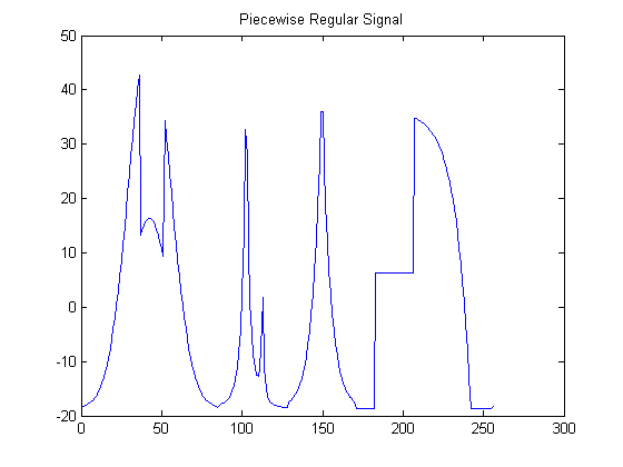
N=256 Piecewise Regular Signal

The output signal is plotted below.

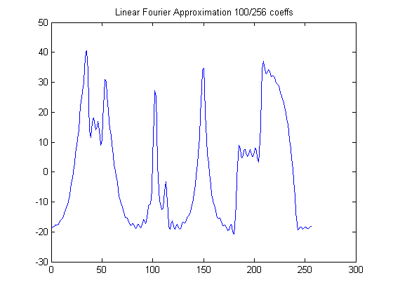
100 coefficients Linear Fourier Approximation

Linear Wavelet Approximation is a bit more involved. Firstly, the input signal is decomposed to a scale \(J\).In this demo, \(J\) is \(4\). Then we retain 100 coefficients starting from the coarsest scale, ie., we start with approximation and detail coefficients at the coarsest scale, then we choose detail coefficients from the next finest scale and so on. In this example, approximation and detail coefficients at the coarsest scale have \(16\) coefficients each. The next finer scale has \(32\) detail coefficients followed by \(64\) at the following one and so on. Since we are choosing \(100\) coefficients , we retain only \(36(=100-16-16-32)\). The rest of the coefficients are set to zero and the inverse DWT is computed in order to reconstruct the signal.The output signal is plotted below

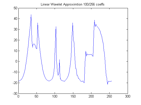
100 coefficients Linear Wavelet Approximation

It can be seen that Wavelet approximation returns a better result with this kind of signal.While linear fourier approximation has a low-frequency bias wavelets tend to capture discontinuities and signal fluctuations at almost every scale which results in better approximation performance.