
Sampling Theorem, Interpolation and Aliasing
This chapter is meant to be a short introduction to Digital Signal processing. Most real life signals exist in analog ( continuous time) domain but from a computational point of view it makes sense to discretize them first. These signals are first sampled and then digitized (sampling along the dependent axis) to convert them to digital signals. The conversion back to analog signal is called interpolation and utilizes a Digital to Analog converter. More on these conversions can be found in references.
Shannon's Sampling Theorem
In order to exactly recover a continuous time signal containing a maximum frequency of \(f_{max}\) , it should be sampled periodically at a rate of \(f_{s} \gt 2f_{max}\). The lower bound on the sampling rate \(f_{s}\) is called Nyquist frequency \(f_{N}=2f_{max}\).
Let \(x(t)\) be the continuous-time signal and \(x(k)\) be the samples of this signal then according to Shannon Interpolation rule \[ x(t)=\sum_{k=-\infty}^{k=\infty} x(k)h(t-kT_{s}) \] where \(T_{s}=\frac{1}{f_{s}}\) is the sampling rate and \(h(t)=\frac{sin(\pi \frac{t}{T_{s}})}{\pi \frac{t}{T_{s}}}\) is a sinc-shaped envelope.
Aliasing
Aliasing occurs when a signal is sampled at a frequency less than the Nyquist frequency, \( f_{s} < 2f_{max}\) which causes higher frequencies [ \( > f_{s}/2\) ] in the signal to appear as lower frequencies and distorts the reconstructed signal. An example of aliasing is shown in the figure. A sampling rate of \(100 Hz\) is set and two sinusoids with frequency components \(30 Hz\) and \(60 Hz\) respectively are sampled with this sampling frequency. Aliasing occurs in the second case and \(60 Hz\) sinusoid appears as \(40 Hz\). This phenomena is also known as folding as the signal appears to be folded back into the lower frequency.
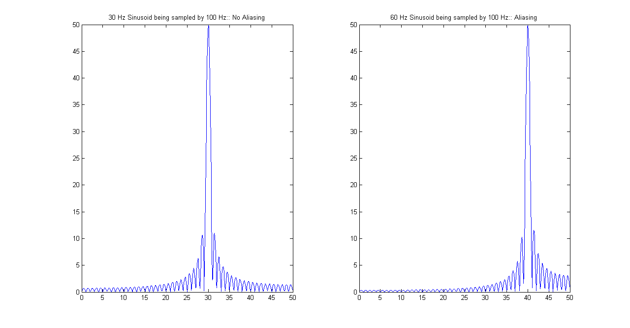
Aliasing Demonstration